| Issue |
Eur. Phys. J. Appl. Phys.
Volume 100, 2025
Special Issue on ‘Imaging, Diffraction, and Spectroscopy on the micro/nanoscale (EMC 2024)’, edited by Jakob Birkedal Wagner and Randi Holmestad
|
|
|---|---|---|
| Article Number | 20 | |
| Number of page(s) | 37 | |
| DOI | https://doi.org/10.1051/epjap/2025018 | |
| Published online | 30 July 2025 | |
https://doi.org/10.1051/epjap/2025018
Original Article
Benchmarking analytical electron ptychography methods for the low-dose imaging of beam-sensitive materials
1
Electron Microscopy for Materials Science (EMAT), University of Antwerp, Groenenborgerlaan 171, 2020 Antwerp, Belgium
2
NANOlight Center of Excellence, University of Antwerp, Groenenborgerlaan 171, 2020 Antwerp, Belgium
3
Department of Chemistry and center for Nanoscience, Ludwig-Maximilians-Universität München, Butenandtstrasse 11, 81377 Munich, Germany
* e-mail: This email address is being protected from spambots. You need JavaScript enabled to view it.
Received:
6
December
2024
Accepted:
23
May
2025
Published online: 30 July 2025
Abstract
This publication presents an investigation of the performance of different analytical electron ptychography methods for low-dose imaging. In particular, benchmarking is performed for two model-objects, monolayer MoS2 and apoferritin, by means of multislice simulations. Specific attention is given to cases where the individual diffraction patterns remain sparse. After a first rigorous introduction to the theoretical foundations of the methods, an implementation based on the scan-frequency partitioning of calculation steps is described, permitting a significant reduction of memory needs and high sampling flexibility. By analyzing the role of contrast transfer and illumination conditions, this work provides insights into the trade-off between resolution, signal-to-noise ratio and probe focus, as is necessary for the optimization of practical experiments. Furthermore, important differences between the different methods are demonstrated. Overall, the results obtained for the two model-objects demonstrate that analytical ptychography is an attractive option for the low-dose imaging of beam-sensitive materials.
Key words: Electron ptychography / beam damage / event-driven detection / low-dose imaging
© EDP Sciences, 2025
 Open Access article, published by EDP Sciences, under the terms of the Creative Commons Attribution License (https://creativecommons.org/licenses/by/4.0), which permits unrestricted use, distribution, and reproduction in any medium, provided the original work is properly cited.
This article is published in open access under the Subscribe to Open model. This email address is being protected from spambots. You need JavaScript enabled to view it. to support open access publication.
1 Introduction
Within recent years, scanning transmission electron microscopy (STEM) has evolved into an attractive tool for the investigation of beam-sensitive objects such as viruses [1,2], 2D materials [3–5], zeolites [6–10], Lirich oxides [11–13], polymers [14], perovskites [15–17] or metal-organic frameworks (MOF) [18,19]. When imaging such fragile materials, the damage following the transfer of energy from interacting electrons [20], such as e.g. knock-on displacement of atoms [21,22], heating [23] or radiolysis [24], imposes a critical electron dose [25] beyond which the specimen structure is lost. This critical dose then constitutes the main experimental limitation, thus in practice determining the best achievable resolution [26,27].
More generally, the prevalence of beam damage requires both a re-evaluation of the maximum electron dose to be invested and an improvement in detector quantum efficiency (DQE). The latter was fulfilled by the introduction of direct electron detectors (DED) [28–38] surpassing the capacities of conventional scintillator cameras [39], including in terms of their modulation transfer function (MTF) [40–42]. The gain in recording speed, allowed by faster electronics, furthermore enabled the acquisition of a convergent beam electron diffraction (CBED) pattern at each scan position [43], a technique often referred to as momentum-resolved STEM (MR-STEM) [44] or 4D-STEM [45]. More recently, event-driven detection [46], based on the Timepix [29,32,36,47] technology, permitted the extension of this technique to sub-microsecond single-pattern acquisition times [48–50], thus reaching the same speed as conventional STEM.
The subsequent knowledge on the far-field intensity distribution furthermore enables the use of a class of computational imaging methods known as ptychography [51–53] for the measurement of the projected electrostatic potential of the illuminated object, in the form of a phase shift map. Those methods consist in the correlative use of a series of coherent scattering experiments, in which a redundancy of imprinted specimen information permits the retrieval of a common illuminated object. They can be thus be considered as an extension of the well-established coherent diffractive imaging (CDI) technique [54–59] to the situation where multiple independent recordings are employed and where, at least in the basic case, no prior information is available.
Among ptychographic methods based on the focused-probe geometry, iterative phase retrieval [60] approaches have recently met some success e.g. with biological specimens [1,61–64]. Those approaches consist in the probe position-dependent simulation of the elastic scattering of the incident electrons, thus leading to a repeated update of the multiplicative transmission function  used to represent the specimen, given the error made against the experimental recordings and while cycling through the corresponding scan positions. This update is performed a number of times for each complete cycle, depending on the chosen batch size, and usually follows one of the several variants [65–72] of the Gerchberg-Saxton algorithm [73–74] for sequential projections or is given by the gradient of a specific loss function [75–78], i.e. the maximum likelihood approach. The process may also include a regularization term [71,79–83] or be based on a parameterization strategy [83–86].
Due to the wide range of parameters available, encompassing e.g. the coupled loss and regularization functions, the update strength, the batch size, the initial guess on the reconstructed object or the possible use of a supplementary momentum term [71], iterative methods possess a high degree of flexibility. On the other hand, while a specific choice of parameter set may permit a degree of adaptation to particular cases, for instance with regards to the noise model [78,87–89], this also implies the need for a complex tuning step to achieve numerical convergence [90]. Different results may otherwise be obtained through separate reconstruction processes or algorithms, hence creating reproducibility issues. Achieving convergence may furthermore prove more challenging in the low-dose case [76,91], where the exploited far-field patterns are underdetermined, independently of the dose-efficiency demonstrated by the converged result in itself. Finally, iterative ptychography remains numerically intensive and often requires advanced computation capacities to avoid exceedingly long processing times [92–96].
For those reasons, there is still a high interest in pursuing work on analytical solutions [97–99] which, since they lead to method-unique results through direct and well-understood imaging processes, arguably constitute more reproducible measurement approaches. In particular, as they are also fast, their application in a wide range of conditions or for large collections of specimens can be streamlined, hence making those methods especially useful for challenging experimental cases. In-line treatment options permitting live imaging [100,101] have been reported as well, while this remains challenging in the framework of an iterative process [102]. Analytical ptychography has moreover demonstrated a high dose-efficiency [103–106], including with a sensitivity to light elements [107–110], and was successfully applied to a variety of beam-sensitive objects [9–14,16] in recent years.
In this publication, the fundamental capacities of analytical ptychography methods to image a beam-sensitive specimen are explored in conditions of very low electron dose. In particular, interest is taken in the resolution achieved for different numerical apertures, in the dose-dependent precision of the measurements and in the fundamental frequency transfer capacity of different approaches. The methods investigated are the Wigner distribution deconvolution (WDD) [98,111–113], integrated center of mass (iCoM) [114,115] imaging as well as the sideband integration (SBI) [99,103,104,116] method, sometimes referred to as single sideband (SSB) [106]. Benchmarking is continued with an overfocused probe [117,118] and an adapted process permitting the direct correction of known aberrations. This specific recording geometry has recently attracted interests for the imaging of beam-sensitive objects and bears similarity with the original idea of ref. [119]. After an initial review of the theory in the fully coherent case, practical implementation is demonstrated through the newly introduced scan-frequency partitioning algorithm (SFPA), permitting a straightforward parallelization and offering high flexibility in the size and pixel resolution of the reconstruction window. All demonstrations made here are based on MR-STEM simulations, hence allowing direct control over the illumination parameters and the dose, while ensuring sparsity in the electron counts. Two model objects are employed: monolayer MoS2 and ice-embedded apoferritin [110].
2 Theory of analytical ptychography and new highly parallelizable implementation
2.1 Coherent and elastic interaction under the phase object approximation
2.1.1 Transmission function
In its conventional form [97,98], analytical ptychography makes use of the phase object approximation (POA) [120]. In this context, the imaged material is considered thin enough so that no variation of wave amplitude occurs within it, thus making the scattering-induced phase shift additive along the propagation axis. For thicker objects, the applicability of the POA is limited due to the role of near-field propagation, leading to a finite depth of focus [121,122] and dynamical diffraction effects such as channeling [123].
Formally, the elastic interaction of the electron probe  with the specimen is then modeled by a multiplication with a transmission function
  , defined for each real-space position
  in the specimen plane by
 (1)
(1)
where  is the projected electrostatic potential of the specimen, i.e. the integral of the three-dimensional potential along the propagation axis. The interaction parameter σ, expressed in V−1 ⋅ m−1, is given by
 (2)
(2)
with e is the elementary charge, m the electron rest mass, h the Planck constant and c the speed of light. The product of σ with  thus represents the local phase shift imposed to the electron wavefunction by the specimen and is typically given in radians.
Importantly, due to the dependence of σ on U, the acceleration voltage affects this phase shift in a non-linear manner, independently of the specimen itself. An empirical absorption term may also be added to  , as an imaginary number, to improve the agreement with experimental results [120,124], e.g. by accounting for amplitude variations in a computationally retrieved transmission function. Typically, this term is related to inelastic scattering [125,126], which otherwise leads to a diffuse component in the far-field [127–130], and specimen vibrations [131–133]. In this work, it is left out for simplicity, i.e. the interaction is assumed to not affect the coherence of the electron beam.
2.1.2 Convergent illumination
Continuing, given a fully coherent illumination, the electron probe  is found equal to
 (3)
(3)
with  the geometrical aberration function and
  representing the aperture in the focal plane of the probe-forming lens, being equal to 1 for
  and 0 otherwise. The quantity qA = sin(α)/λ introduced here is the reciprocal space cut-off imposed by the aperture, with α the semi-convergence angle and λ the relativistically corrected wavelength [134]. Noteworthily, the aperture function actually used in the numerical implementation is further normalized, as being representative of the wavefunction in the focal plane.
The notations ℱ and ℱ−1 respectively refer to a Fourier transform and an inverse Fourier transform, given by
 (4)
(4)
with Fourier normalization left implicit.
2.1.3 Scattered and measurable intensity
At a given scan position  , a localized exit wave
  is formed which is given by
 (5)
(5)
hence the diffracted intensity  accessible in the far-field, with
  a scattering vector, is
 (6)
(6)
As such, this quantity is interpretable as a probability distribution among the locations, at the concerned optical plane  , for the collapse of the electron wave.
Finally, the intensity  measured by the camera, across detector space
  , includes a possible point spread effect represented by the MTF
  ,
,  being the reciprocal dimension of
  . This leads to
 (7)
(7)
Given that  is a real quantity, if the MTF-induced information spread effect is isotropic, then
  and
and  are both real and point-symmetric. This assumption is implicit in the rest of this work.
2.2 Wigner distribution formalism
2.2.1 Scattering data reformulation
Given the prior recording of  through an MR-STEM experiment, a Fourier transform with respect to the scan coordinates
  towards an arbitrarily sampled spatial frequency space
  leads to a complex distribution
  . As long as real-space is sampled finely enough by the scan points
  , i.e. under the condition of sufficient overlap ratio
  between successively illuminated areas [135],
  can then be interpreted as a map of the specimen-dependent
  -responses attributed to the camera pixels
  . In particular, each scattering vector
  in the far-field is assimilated to a single conventional TEM image by arguments of reciprocity [136,137]. More details on the redundancy condition and area overlap are provided in Appendix A, including with a mathematical criterion.
The distribution  is found equal to
 (8)
(8)
where  and
and  are Wigner distributions [138], i.e. autocorrelations of the probe and of the transmission function.
Formally, they are given by
 (9)
(9)
and
 (10)
(10)
The function  encompasses the imperfections in the illumination and is equal to
 (11)
(11)
As such, the insertion of this term in a ptychographic processing allows correcting for geometrical aberrations.
A subsequent inverse Fourier transform from the camera dimensions  to an arbitrary set of reciprocal real-space coordinates
  leads to
  , a new complex four-dimensional distribution, equal to the product of the Wigner distributions with the MTF, i.e.
 (12)
(12)
2.2.2 Wigner distribution deconvolution and direct extraction of the transmission function
The WDD method for analytical ptychography [98–113] thus first consists in the recovery of  through
 (13)
(13)
where ϵ is a small number introduced to avoid divisions by zero, i.e. the actual deconvolution is done via a Wiener filter process [139]. Noteworthily, a careful choice of the Wiener parameter ϵ is also important to avoid an amplification of the noise propagated from detector space [106].
As a second step in the processing, the summation of  along
along  permits the recovery of the transmission function by
 (14)
(14)
where  is introduced as an intermediary result. With the deconvolution done,
  , i.e. the measurement of the phase shift map
  by WDD ptychography, can be obtained from
  by extracting its angle. In most practical cases, including those presented here, the values obtained remain small enough to avoid phase discontinuities, thus making an unwrapping process unnecessary.
2.2.3 Zero-frequency component
As illustrated by equation (14), the measurement is performed such that  . Consequently,
  is a real number, which implies that the mean of the ptychographic phase in the reconstruction window, i.e. its DC component, remains inaccessible. This is consistent with the fact that phase, as a mathematical abstraction rather than a significant physical quantity, remains unmeasurable unless compared to a reference, e.g. by wave interference like in the case of off-axis electron holography [140,141].
In particular, in the coherent and elastic interaction regime, only relative local phase shifts created within the illuminated patch, thus requiring gradients in the specimen-induced phase shift map, can lead to measurable changes in the momentum distribution [142]. As a side-note, the normalization of  by the real constant
  only modifies its amplitude, and not its angle. It thus does not affect the measurement of the projected potential itself.
2.2.4 Resolution limit
Continuing, since  for
for  , owing to formula (10), it appears at first sight as though the best resolution achievable by the WDD approach is equal to half the conventional Abbe criterion δrAbbe = 0.5/qA. In reality, super-resolution, i.e. the transfer of frequencies exceeding the 2qA diffraction limit [74,98,143–146], is still possible based on the so-called stepping out method [98,113].
This is nevertheless done at a high cost in dose [147], as it is specifically dependent on the availability of dark field electrons. Since this publication focuses particularly on the dose-efficiency of analytical ptychography, this aspect is left for future work. The WDD method can otherwise make use of the dark field electrons outside of the stepping out paradigm, as apparent in the equations. Moreover, and as long as the interaction can still be faithfully described using the POA, geometrical aberrations are corrected through the introduction of the term  , defined in equation (11).
2.3 Sideband formalism for a weak scatterer
2.3.1 Simplification of Wigner distribution formalism via a first order Taylor expansion
The special case where the specimen can be considered weakly scattering, in addition to fulfilling the POA, occurs when the range of phase shift covered by the measurable  , i.e. accounting for the reduction due to resolution limit, is significantly smaller than 1. Equivalently to the well-known small-angle approximation, the transmission function may be then replaced by the following first order Taylor expansion
 (15)
(15)
This condition is usually referred to as the weak phase object approximation (WPOA) [120].
It then follows that
 (16)
(16)
As the condition of a weakly scattering object also implies that  , equation (8) leads to
 (17)
(17)
Notably, this is also justified by the realness of  , which implies that
  .
.
The functions  and
and  are given by
 (18)
(18)
 thus consists of a zero-frequency term, associated to the unscattered portion of the electron beam, and a two-sideband term resulting from the Fourier transform of the distribution
  .
.
2.3.2 Deconvolutive extraction of the potential
Equation (17) serves as a basis for the sideband method of analytical ptychography [99,103,104,116], in this work referred to as SBI. It can thus be understood as a special case of the Wigner distribution approach, applicable when the object fulfills the WPOA. Here, a deconvolutive form is used, similarly to e.g. reference [116]. For clarity, it will be referred to as SBI-D in the rest of this text, while the conventional summative form [103,104] will be referred to as SBI-S.
The SBI-D process thus consists in performing
 (19)
(19)
 is an intermediary result and
  is introduced for normalization, i.e. the projected potential is obtained by calculating a mean among the scattering coordinates
  , post-division by
  .
.
Importantly, like for the WDD case, the DC component is not recoverable, since  , as is shown by formula (18). The inclusion of
  also permits the correction of aberrations, at least as long as the WPOA is fulfilled.
2.3.3 Summative extraction of the potential
If the influence of the MTF is neglected, i.e.  , then equation (17) becomes
 (20)
(20)
Hence,  can be described as a superposition of two sidebands terms with a zero-frequency component.
In practice, this sideband-like geometry means that, upon visualizing the values across the  -dimensions, for a given specimen frequency
  and as long as
  , the double overlap area will be homogeneously equal to
  . This constitutes the basis of the conventional SSB workflow [103,104] and provides an opportunity for straightforward aberration correction [107,148].
In this context, the SBI-S process consists in performing a summation within the double overlaps, while excluding triple overlaps where the terms cancel out. Formally, it consists in
 (21)
(21)
where the  terms are given by
 (22)
(22)
Each thus aims to access one of the double overlap areas within the  distribution, with a phase shift term inserted to compensate aberrations.
2.3.4 Phase contrast transfer function
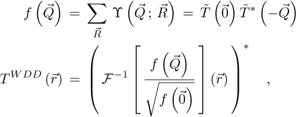
The contrast transfer function (CTF)  , depicted in Figure 1, is introduced due to the summation over
  and is given by
 (23)
(23)
As such, it is equal to the surface of the double overlap region, across camera space  , corresponding to each spatial frequency
  . It is interesting to note that, while this CTF is peaked at intermediary frequencies, i.e. close to qA, it decays for both higher and lower frequencies.
Here, it should be furthermore highlighted that, while the CTF of SBI-S is explicit, SBI-D possesses the same fundamental characteristics with regards to frequency transfer, as shown by the dependence of  on
on  . In essence, it is not the choice between the summative or the deconvolutive forms that leads to the frequency weighting, but rather the assumption of a weakly scattering object in itself.
In particular, if equation (20) is fulfilled, and if no geometrical aberrations are present, the parts of the distribution  found outside the double overlap areas are expected to carry no useful information on the specimen, and thus to contain only noise.
  then reflects the information content in the scattering data itself, being equal to the proportion of available scattering vectors
  that are useful to recover a specific frequency component
  of the specimen, i.e. it constitutes the phase contrast transfer function (PCTF) of the experiment in the sense of e.g. reference [104]. When the WPOA is fulfilled, it is thus expected to intrinsically apply to all STEM-based phase retrieval methods, irrespective of whether their formulation assumes a weakly scattering object in the first place.
As such, the SBI method, which consists in a treatment based explicitly on equation (17), permits to exclude all pixels outside double overlaps, thus in principle minimizing the total noise in the real-space result. As explained in details in reference [149], the SBI-based treatment of counts in the detector space  , which follow Poisson statistics [150], then leads to a predictable noise level added to the frequency spectrum of the recovered object, given by the square root of the PCTF.
In this context, the option to deconvolve the reconstructed phase shift  post-process with
  has been proposed as an effective noise normalization strategy [106,149], i.e. rendering the noise level homogeneous across spatial frequencies. Deconvolving by the complete
  , which in the conventional SSB workflow [103,104] is equivalent to averaging
  within the double overlap areas instead of performing a summation, may otherwise permit to homogenize frequency transfer. This is nevertheless only practical when the dose is high enough, as the amplitude of the frequency components to be amplified may then be below the noise level.
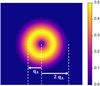 |
Fig. 1 Depiction of the PCTF |

2.3.5 Applicability of the weak scatterer approximation
It should be understood that the specific situation where  possesses the low value range of a weak phase object only occurs in a handful of cases. This may not only be due to excessive atomic potentials or material thicknesses, but also because lower acceleration voltages U imply non-linearly higher values for the interaction parameter σ, as shown by equation (2). In the case where the illuminated object is not a weak scatterer, as noted e.g. in reference [106,151], the SBI process still imposes a frequency-wise attenuation following
  , due to the forms of
  and
and  . The CTF is then method-induced rather than reflective of the PCTF of the experiment itself.
In this situation, the underlying sideband-like geometry in the distribution  also cannot be expected to occur strictly, i.e. the values taken by
  -coordinates within the
  -wise double overlap areas may not be homogeneously equal to
  anymore and exploitable information may be present outside as well. On that second aspect, it is noteworthy that, under the more general POA, non-zero coordinates of
  include both the triple overlap areas and the dark field. In contrast, the scattering of electrons outside the primary beam is not possible in the framework of the WPOA, as directly noticeable in equations (17) and (20). Whereas this is not the case for the iCoM and WDD methods, the SBI-S and SBI-D processes are thus unable to exploit dark field electrons.
As a side-note, the CTF  leads to artificial image features, e.g. negative halos around atomic sites [152]. If the specimen is not weakly scattering, such artificial features are not expected to occur through methods based only on the POA, hence demonstrating the possible violation of the WPOA upon comparison of results.
2.3.6 Interests of the deconvolutive approach
Finally, when comparing the two forms of sideband ptychography, SBI-D presents a few advantages compared to the already established SBI-S approach. First, the MTF  can be explicitly included. Second, SBI-D permits the use of an arbitrarily shaped aperture [116] where the selection of specific overlapping regions would be less obvious, and thus the straightforward application to specific phase plate designs [153–155].
2.4 Center of mass imaging
2.4.1 Scan position-wise average momentum transfer
The center of mass (CoM)  of the scan position-dependent CBED patterns constitutes a measurement of the average momentum transfer between the scattered electrons and the specimen. Under the POA, the CoM is linearly related to the local gradient of the projected potential [114]. Formally, this means that
 (24)
(24)
with  a CTF given by
 (25)
(25)
 is depicted in Figure 2. This CTF is peaked at low frequencies and smoothly decays as a function of
  , thus indicating difficulties in transferring higher frequencies.
In the absence of a fast DED to perform an MR-STEM experiment, the average momentum transfer is conventionally approximated by using quadrants of a segmented detector [156,157], a technique usually referred to as differential phase contrast (DPC) in relation to historical references [158,159]. In that context, CoM imaging can be understood as a more accurate approach to measuring the DPC signal [44], in particular considering that the use of segmented detectors leads to a non-isotropic CTF [160]. As a side-note, another existing detector paradigm consists in a position-sensitive non-pixelated design [161].
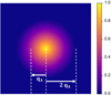 |
Fig. 2 Depiction of the OTF |

2.4.2 Fourier-based extraction of the potential
Following the measurement of  , an extraction of the projected potential can be performed through a simple Fourier integration scheme, as conventionally used e.g. for the integrated DPC (iDPC) [115,162] counterpart to iCoM. This consists in
 (26)
(26)
with  an intermediary result. Importantly, just like for the WDD and SBI methods, the DC component is inaccessible, as shown by the scalar product with
  .
.
Importantly, in contrast to analytical ptychography, aberration correction does not seem straightforward with CoM imaging. The dependence on focus and thickness has nevertheless been investigated in recent years [163–167], in particular with the objective of maintaining an interpretable contrast when the POA is not strictly fulfilled anymore.
2.4.3 Optical transfer function
Continuing, in contrast to the PCTF  , which is applicable in the situation where the WPOA is fulfilled and is then reflective of the information content of the scattering data itself,
  is fully process-induced and is derivable in the more general context of the POA. In particular, it is equal to the Fourier transform of the unaberrated probe intensity [114] and, as such, can be termed as an optical transfer function (OTF) in the sense of [168]. Beyond that, the immediate consequence of this OTF is the higher weighting of low-frequency features, compared to the rest of the object spectrum, being then attenuated.
As a result, the iCoM imaging mode is prone to low-frequency artefacts [162], which may constitute a limit to the use in the low-dose case [169]. This is nevertheless not problematic for many of the common applications of DPC and CoM consisting in the imaging of long-range features, such as e.g. charge density gradients [170], magnetic domain structures [171], large proteins [2], interfaces between materials [172], particle shapes [173], skyrmions [174] or stray electrostatic fields [175].
In principle, and like in the SBI case, it should furthermore be possible to compensate this effect by directly deconvolving the real-space result with  , though the limitation is then whether the frequency components to be amplified have been brought below the noise level. Hence, such a solution is not practical at low doses. In the specific situation where iCoM imaging is employed on a weak phase object, both the PCTF
  and the OTF
  can be expected to apply.
2.5 Scan-frequency partitioning algorithm
Algorithm 1 SFPA
1: Choose imaging method
2: Partition  -coordinates in packets
3: Define  -grid
-grid
4: Partition  -coordinates in domains
5: if imaging method is WDD then
6: Initialize intermediary result as 
7: else if imaging method is SBI-D then
8: Initialize intermediary result as 
9: else if imaging method is SBI-S then
10: Initialize intermediary result as 
11: else if imaging method is iCoM then
12: Initialize intermediary result as 
13: Distribute  couples asynchronously
14: for each packet  do
do
15: for each domain  do
do
16: if imaging method is WDD then
17: Calculate 
18: Calculate 
19 Add  to
to 
20: else
21: Calculate 
22: if imaging method is SBI-D then
23:Calculate 
24: Add  to
to 
25: else if imaging method is SBI-S then
26: Calculate 
27: Add  to
to 
28: else if imaging method is iCoM then
29: Calculate 
30: Add  to
to 
31: if imaging method is WDD then
32: Divide  by
by 
33: Inverse Fourier transform along 
34: Transmission function is measured
35: Extract angle of transmission function
36: Phase shift map is measured
37: else
38: Inverse Fourier transform along 
39: Phase shift map is measured
2.5.1 Motivations and numerical basis
One of the main limiting factor for the practical implementation of analytical ptychography is the necessity to first load the full dataset in computer memory, in order to perform a collective treatment consisting in a succession of fast Fourier transforms (FFT) and deconvolution/summation steps. Such a process requires a large available memory and makes e.g. GPU implementation difficult. This publication thus proposes a new scan-frequency partitioning algorithm, i.e. the SFPA solution mentioned in the introduction, which constitutes a straightforward, memory-limited and parallelizable implementation of the WDD, SBI and iCoM methods. As explained in more details below, this approach also relaxes sampling conditions that would normally be imposed by the scan grid.
The basis for the algorithm is the replacement of the FFT leading from the scan dimension  to the spatial frequencies
  with an explicit, term-by-term, summation, e.g. following the Einstein notation. This is conventionally referred to as the einsum algorithm, as included e.g. in several Python packages. A similar explicit construction of the Fourier series was used for instance in ref. [100] for live processing. The formal procedure is described in the following paragraphs, and is otherwise provided in Algorithm 1. Noteworthily, under the current implementation developed for this work, the PyTorch package [176] was chosen for its capacities in straightforward GPU-based programming.
2.5.2 Partitioning of calculation steps
The SFPA encompasses two distinct levels of partitioning among the calculation steps needed for the complete process. A first one is ensured by cutting the complete four-dimensional dataset  in packets of scan positions
  , each containing a user-defined number of arbitrarily chosen coordinates
  . The packets are treated individually, in particular the einsum-based Fourier transform, itself done for specific spatial frequency domains
  . This then represents the second partitioning introduced in the algorithm.
The complete set of calculations is thus divided in a number of single independent operations, each involving a specific  couple. Those operations yield partial Fourier transformed datasets given by
 (27)
(27)
depending on the type of reconstruction performed, i.e.  is the input of a WDD process while
  is needed for SBI and iCoM. Note that in equation (27), the term ℱ−1 indicates an inverse Fourier transform done over the camera space, for the few CBED patterns in
  .
.
Each partial Fourier transformed dataset is used for one of the following calculations
 (28)
(28)
where the packet-specific intermediary result  is obtained through equations (13) and (14),
  through equation (19),
  through equation (21) and
  through equations (24) and (26). Performing the same process for the entirety of the
  -to-
-to- components of the Fourier series finally yields the full reconstruction result.
Noteworthily, in the case of the WDD method, the complete, four-dimensional, Wigner distribution  is not explicitly retrieved. Instead, in the implementation described by Algorithm 1, each
  couple leads to an increment of
  directly. The same einsum-based Fourier transform strategy could nevertheless be used for this purpose, i.e. without an immediate summation step across
  , straightforwardly as well.
2.5.3 Opportunity for parallelization
A first interest of the scan-frequency partitioning algorithm is its low need in active memory, since the size of the packets  and domains
  are chosen by the user directly. This in turn permits to adapt the process to the computer memory available, including as part of a straightforward implementation on a GPU, e.g. involving specialized Python-based procedures [176]. Furthermore, since the treatment of each individual
  couple is independent of all others, parallelization is possible along both the
  and
and  dimensions. In comparison, the implementation reported in reference [100] only allowed it along
  , though it was already enough for live processing using a computer with sufficient performance.
Given the low memory requirement of a single  calculation, such a parallelization strategy is in principle implementable on a wider range of devices, including low-end. Though extensive numerical benchmarking was left for future work, it should be noted that avoiding the two-dimensional
  -to-
-to- FFT can be expected to lead to an increment in the numerical complexity of the complete process. Specifically, it then goes from the typical O (Ns;x ⋅ Ns;y ⋅ log(Ns;x ⋅ Ns;y)) to
  , with Ns;x/Ns;y the number of positions along the two scan axes and
  the total number of frequencies
  used. This number is equal to
 (29)
(29)
where π (2qA) 2 is the reconstructed frequency surface and Srec is the reconstructed real-space surface. Specifically, the discretized frequencies  are distributed within a disk of radius 2qA, with a pixel density determined by the real-space extent of the reconstruction window.
Note that, in order to avoid aliasing and periodicity artefacts, Srec has to be made sufficiently larger than the scanned surface S, with a portion of it maintained at a value of zero in the real-space reconstruction window. The same is true in the frequency space window [177]. Overall, the preparation of the reconstructed object in both  - and
- and  -space follows the conventional approach used, for instance, in typical multislice simulations, as is described e.g. in reference [178].
2.5.4 Decorrelation of scan and reconstruction grids
Perhaps most importantly, and as implied by equation (29), the employment of the einsum algorithm permits the explicit decorrelation of the scan and frequency dimensions. As such, the real-space reconstruction grid, and thus the actual choice of  -coordinates for which the result is calculated, is prepared independently of the scan grid, and the formal contribution of each given
  -coordinate to a single arbitrary frequency
  may be determined separately from all others. In contrast, in the conventional full FFT solution [103,113], as well as in reference [100], each scan point equates one pixel in the result. The SFPA however permits a calculation at frequencies exceeding e.g. the maximum that would then be allowed by the finite scan interval. In that context, it becomes possible, for instance, to perform a reconstruction given a strongly defocused probe and less scan positions [118], while conserving an appropriately resolved reconstruction window in real-space.
At first sight, this development may be understood as breaking the Nyquist-Shannon sampling theorem. The possibility of retrieving information beyond the Nyquist frequency of the scan grid should however be seen as resulting from the usage of the information available along the  dimensions. In particular, in defocused conditions, the amount of details contained in the far-field intensity is greater as it then consists in a shadow image of the specimen [179]. As such, including the appropriate aberration function in
  permits to correctly translate this information back into the result and extend the area, in the real-space reconstruction window, that may be informed by a single scan position. Beyond this, since such a measurement geometry is already commonly used in combination with iterative approaches [117,118], where a similar decorrelation of the scan and reconstruction pixels is implicit and where the same scattering data is used, this fundamental ability of analytical ptychography is expected.
Another interest of using an arbitrary set of reconstruction frequencies is the facilitated implementation of high-pass and low-pass filtering, as the concerned  -coordinates can be omitted from the calculation, hence reducing
  as well. A limitation to this practice is however that, in order to perform an extraction of the phase shift map from the WDD-retrieved transmission function, it should have a defined zero-frequency component, i.e. the mean of the complex numbers
  should not be equal to zero. For this reason, only the inherent high-pass filtering, and not both the high- and low-pass ones, may be used for the SFPA-based WDD calculation.
The employment of an orthonormal Fourier transform may moreover be useful in ensuring appropriate numerical normalization, as the number of pixels in the reconstruction grid and the scan grid are likely to differ. This proper choice of convention is important to conserve consistent results among slightly different scan grids among recordings.
Finally, the operations involving the dimensions  and
and  , as in equations (14), (19), (21) and (24), are performed in the camera space. As such,
  represents a spatially limited kernel, similarly to e.g. reference [70], in which numerical artefacts are prevented by a simple interpolation or zero-padding step. In that manner, the process can also precisely account for elliptical distortions observed in the far-field pattern [180] and prevent them from affecting the result, based on an initial calibration of the
  dimension [166].
3 Atomic-resolution imaging of MoS2
3.1 Conventional focused-probe conditions
3.1.1 Simulation and processing parameters
In order to test the dose-efficiency of the iCoM, SBI-D and WDD methods in the conventional focused-probe, high-resolution, condition of electron ptychography, an MR-STEM simulation was performed based on a monolayer MoS2 specimen, for which the POA can reasonably be considered fulfilled. Diffraction patterns were calculated in a scan grid of 64 by 64 points, covering an area of 2 nm by 2 nm, hence with an interval of about 32 pm. Illumination conditions were chosen as representative of the capacities of a modern aberration-corrected microscope such as e.g. a Titan Themis 60–300 (Thermo Fisher Scientific). Specifically, the acceleration voltage U and the semi-convergence angle α were assigned values of 60 kV and 30 mrad respectively which, for reference, leads to a Rayleigh criterion δrRayleigh = 0.61/qA of about 99 pm. As illustrated in Figure 3, the optical conditions described above lead to an area overlap  between two scan points neighboring each other along a scan direction, and 62.3% along the diagonal.
  is defined for higher distances
  as well. This highlights that a degree of redundancy remains beyond immediate neighbors, which is exploited by the ptychographic process as well. More details on the calculation of the area overlap and how it differs from the conventional approach [135] can be found in Appendix A.
Continuing, the propagation of the electron wavefunction through the specimen was modeled based on the multislice approximation [181–183] and the atomic potentials were calculated using parameterized hydrogen orbitals as described in reference [184]. The specimen potential was sliced below the atomic plane level and pixelated such that a maximum scattering vector of up to twice the range actually used could be included. Thermal motion within the lattice was accounted for by repeating the calculation for a total of 64 configurations of random lateral atomic shifts, and averaging the resulting distributions  . The random shift vectors were determined using the frozen phonon approximation [185,186] based on the Einstein model, i.e. assuming non-correlated atomic vibrations [187]. For simplicity, and also because this work aims at reproducing results obtainable with a Timepix3 chip [32,47] at a low acceleraton voltage U, thus in a condition where multiple counting is unlikely to occur [41,48,188], the simulation did not include an explicit MTF. As such, the values taken by the
  function, included in practice in the SBI-D and WDD calculations, only encompassed the role of the finite pixel size of the simulated camera, as implied by the kernel size.
The results of the iCoM, SBI-D and WDD processes, implemented using the SFPA approach described in Section 2.5, are depicted in Figure 4. Specifically, the measurements of the projected potential, expressed in V⋅nm, are shown alongside the square roots of the corresponding Fourier transform amplitudes, for visualization of Fourier weightings along the two-dimensional  coordinates. The calculations were done for a variety of average numbers of electrons per pattern
  and consequent doses D given in e−/Å2. To better highlight the non-linear relation between dose and contrast,
  was given values of 2
l
with l ∈ [2, 3, ..., 10]. Dose-limitation was ensured by repeated random pixel selection, with the number of repetitions being probabilistically determined across the scan window by Poisson statistics. As such, the propagation of Poisson noise from detector space to the reconstruction window can be straightforwardly reproduced, while conserving a realistic sparsity in the scattering frames [105]. This approach is described in more details in Appendix B, alongside its wider interests.
was given values of 2
l
with l ∈ [2, 3, ..., 10]. Dose-limitation was ensured by repeated random pixel selection, with the number of repetitions being probabilistically determined across the scan window by Poisson statistics. As such, the propagation of Poisson noise from detector space to the reconstruction window can be straightforwardly reproduced, while conserving a realistic sparsity in the scattering frames [105]. This approach is described in more details in Appendix B, alongside its wider interests.
Furthermore, for each dose-limited case, the generated sparse diffraction patterns were individually normalized by their sum, pre-treatment. This strategy was adopted for all reconstructions presented in this work and was chosen following the suggestion of reference [149]. This is equivalent to varying the normalization of the wavefunction, scan point-wise, to match the number of counts in each corresponding pattern. Importantly, taking this normalization choice into account will be required for any theoretical estimation of measurement precision in future work, as it leads, in effect, to a change in the variance of single patterns. This solution differs from the usual quantitative STEM approach [189,190], which would have consisted in uniformly normalizing by  . Finally, the
  case corresponds to the direct use of the simulated
  , where the intensity is implicitly normalized. The corresponding result can thus be understood as representing the experimental situation where the best achievable dose-dependent precision is reached, and hence where the noise level is negligible.
As a side-note, in the case of the WDD process, the projected electrostatic potential is obtained through a prior extraction of the phase shift map. Given that the [− π ; + π] range was not exceeded, no discontinuities were observed and thus no unwrapping was necessary.
 |
Fig. 3 Depiction of the overlap ratio |


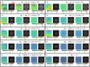 |
Fig. 4 Results of analytical ptychography of monolayer MoS2, applied on the multislice electron diffraction simulation presented in Section 2.1. Calculations are done for a variety of average numbers of electrons per pattern |


3.1.2 Noise level in the micrographs
For the three methods, atomic patterns are already visible from  , hence with a dose below D = 81.92e−/Å2. Moreover, frequencies belonging to the specimen lattice are observed even in the Fourier transforms of results obtained given
  . This first remark is particularly interesting for future applications of electron ptychography to beam-sensitive objects, as it empirically shows what is the true requirement in terms of dose, given a perfectly stable and coherent imaging system. As
  increases, the noise level in the images lessens and specimen frequencies become more dominant compared to the noise background. Such a dose-dependent precision in ptychographic computational imaging has been investigated empirically in the literature [76,88,91,191], as is done here as well, and its lowest achievable value can in principle be predicted by parameter estimation theory [192–197], in particular using the Cramér-Rao lower bound (CRLB) [198].
In this publication, the true frequency-dependent CRLB is not provided since, unless some simplifications such as the WPOA [195,196] are introduced, its formulation remains specific to the specimen [193,194]. The establishment of a general  -dependent metric, which would be dependent on the complete set of experimental parameters, is thus left for future work. Beyond that, the approximation made in reference [197], provided below, leads to a single number CRLBRS representing the minimum standard deviation among distinct measurements, as induced by the propagation of Poisson noise [150], upon retrieving the phase shift map
  in real-space. While it was derived in ideal illumination conditions which are not met here, e.g. the total illumination is not strictly restricted to the scanned area, this metric remains useful to establish a fundamental understanding of the concept.
 (30)
(30)
 represents the total number of probing electrons, while Ns is the total number of scan positions used. S is the surface covered by the scan window, necessarily smaller than the surface Srec as explained in Section 2.5. The number
  of reconstructed frequencies was otherwise described by equation (29), and can here be understood as the number of useful pixels in the reconstruction. A “–1” term is added to account for the unmeasurable DC component. Given that the term 0.5/S is likely to be negligible compared to 2πqA2, CRLBRS shows rather clearly that, in order to achieve a certain goal in measurement precision, the dose D has to be adapted to the aperture radius qA, and thus implicitly to the spatial resolution [199].
3.1.3 Fourier ring correlations
In order to pursue the analysis further, Fourier ring correlations FRC m (k) [200,201], shown in Figure 5, were calculated from the projected potential results through
 (31)
(31)
k is a spatial frequency modulus and Rk = [k − δk ; k] is the corresponding annular domain, with δk a case-dependent precision.  is the Fourier transform of the measured projected potential, for the specific
  case. In this context, the calculated FRC can be interpreted as a frequency-wise measurement of the dose-dependent precision of each method, and thus provides a straightforward dose-efficiency metric. The closer FRC
m
(k) is to 1, for a given spatial frequency modulus k, the closer the corresponding Rk range of the signal is to reaching the best achievable precision. In this example, and for better visibility, the FRC curves are provided in a reduced selection of
case. In this context, the calculated FRC can be interpreted as a frequency-wise measurement of the dose-dependent precision of each method, and thus provides a straightforward dose-efficiency metric. The closer FRC
m
(k) is to 1, for a given spatial frequency modulus k, the closer the corresponding Rk range of the signal is to reaching the best achievable precision. In this example, and for better visibility, the FRC curves are provided in a reduced selection of  , for iCoM in Figure 5a, SBI-D in Figure 5b and WDD in Figure 5c.
A few observations can immediately be done from the calculated FRC. For all imaging modes, three peaks are observed, close to 0.5,1.0 and 1.5 times qA, as well as an emerging fourth one. Those correspond to the hexagonal pattern of spatial frequencies belonging to the specimen, mirroring scattering orders of the atomic lattice, as observed in the Fourier transforms of Figure 4 as well. At the level of the peaks, perfect precision is reached at a much lower  than in the rest of the k-axis. From a naive standpoint, this already tends to show that frequencies
  actually carrying information on the specimen are reconstructed much more efficiently than those containing no information, and which then end up reaching
  at infinite dose. This is expected in a situation where the spectrum of the illuminated object is sparse. In particular, ptychographically processed electrons end up contributing only to the recovered projected potential, i.e. its associated
  -coordinates. This remains true as long as the illumination characteristics are known and no artefactual features are introduced, e.g. from an inaccurate interaction model.
In this context, if one considers the overall calculation as an additive inclusion of single counts' contributions to the measurement, with no question of normalization, the signal-to-noise ratio at  -coordinates belonging to the specimen is expected to directly improve for each dose increment, while the noise level at other frequencies remains the same. The reduction of the background noise is then due to the normalization, and thus occurs at a lower rate than the retrieval of specimen information in itself. Continuing, upon comparing the three frequency peaks mentioned above, it is also noticeable that FRCm (k) ≈ 1 occurs with more difficulty as k increases, i.e. higher values of
  appear more dose-expensive at first sight. The practical reason for it is that the surface covered by an Rk ring increases with k, which thus implies a larger proportion of background noise compared to specimen frequencies. Similarly, the lower values of k lead to a less visually stable value of FRC, due to the low number of actual pixels in the corresponding Rk.
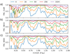 |
Fig. 5 FRC calculated from the |


3.1.4 Contrast transfer capacities
Arguably the most important information to draw from Figure 5 is that, among the three investigated methods, the overall FRC profiles are rather similar. This is of particular interest, as it shows that, for a given frequency component, the dose-efficiencies of iCoM, SBI and WDD are more-or-less the same, in that they reach the best achievable result with comparable dose requirements. As such, what differentiates those imaging modes with regards to the measurement precision in real-space, and in particular to the noise background formed as a function of spatial frequency [149], is the existence of the CTF  for iCoM and
  for SBI, displayed in Figures 2 and 1. Whereas those CTF lead to visually different micrographs, as is directly noticeable in Figure 4, the attenuation of frequency components also contribute to noise filtering. Consequently,
  appears slightly, but noticeably, less noisy than
  , e.g. for
  . This is specifically related to the existence of high-frequency noise, as observed in the Fourier transforms of the WDD results, which is otherwise eliminated by the deconvolutive SBI process.
Beyond that, the underlying difference in the real-space measurement, between the two analytical ptychography methods, consists in an exaggerated dark halo around atomic sites, clearly visible at higher doses and only present in the SBI-D results. This feature is associated to  [152], which is thus shown to not intrinsically apply to the WDD result. As was explained in Section 2.3, this then constitutes a clear indication that the specimen is not a weak scatterer, i.e.
  cannot be considered to constitute the PCTF of the experiment in general. Specifically, the WDD process only assumes the more general POA, here remaining reasonable, and should not be generally expected to show the specific frequency transfer met in the case of a weak phase object. The formulation of the SBI method, on the other hand, is still based on this assumption and will thus have
  as a CTF in any case. Note that the violation of the WPOA is here further confirmed by the range of values covered by the WDD phase shift map, which is above 1.0 rad, as well as by the ground truth of the projected potential, for reference depicted in Figure 6 in a limited real-space window.
More fundamentally, the nonfulfillment of the WPOA means that, in the  distribution, the general sideband-like geometry arising from a weakly scattering specimen is not met in practice. As a consequence, this is not just noise, e.g. in the triple overlap areas, that is removed by the SBI process, but also potentially useful information on the specimen itself. This can be verified in Figure 4 as well, where the Fourier components of
  , at high
  values, are visibly higher than those of
  . This thus leads, in addition to the absence of the artificial features mentioned above, to a slightly better resolution in the WDD measurement.
In parallel, the iCoM imaging mode is affected by the OTF  , whether the PCTF
  of a weak phase object is applicable or not. As such, the higher weighting of low frequencies, with the rest of the spectrum being then attenuated, increases its susceptibility to long-range artefacts [162,169], as explained in Section 2.4 Consequently, low-frequency noise remains dominant up to e.g.
  . This is verified by the Fourier transforms as well.
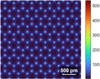 |
Fig. 6 Laterally limited view of the vertical projection of the three-dimensional potential used for the simulation presented in Section 2.1. The quantity is expressed in V⋅nm and is represented in the absence of atomic vibration, i.e. the atoms are all exactly at their rest positions. |
3.1.5 Phase shift value range
Continuing with the projected potential maps displayed in Figure 4, one last remark remains to be made. In high dose conditions, the range of values obtained with WDD is about twice larger than it is with iCoM and SBI-D. This is not due, for instance, to a normalization issue, as the WDD result is obtained by extracting the angle of the initially retrieved transmission function. Furthermore, as is shown in Section 3, the opposite situation can be met as well and, as proven in Section 2.2, the aberration function plays a role too. This thus points out the mismatch in value range as being a fundamental feature of the imaging method rather than a numerical issue. In that respect, it is also worth noting that such a mismatch was observed previously in the literature [106,108,169] as well. Finally, the effect is likely amplified by the higher resolution of the WDD reconstructions, itself due to the better transfer of high frequencies, leading to stronger atomic peaks in the image.
3.2 Overfocused illumination conditions
3.2.1 Simulation and processing parameters
To test analytical ptychography methods in overfocused illumination conditions, a second simulation was performed in the same conditions as described in Section 2.1, though with an added defocus of 40 nm, and only 16 by 16 scan positions leading to an interval of about 133 pm in the scan grid. The simulation and reconstruction windows were enlarged to avoid artefactual probe self-interference. Noteworthily, the reconstruction of frequencies exceeding the maximum that is allowed, in principle, by the scan interval [103,113] is enabled by the SFPA solution described in Section 2.5.
The illumination condition leads to  between neighboring scan points, as shown in Figure 7. Whereas this somewhat high area overlap was found to be fully sufficient for the reconstruction, another attempt with only 8 by 8 points in the same region, which would have permitted 85.7% of overlap, was found to be insufficient. Empirically, this need for a significant value of
  is expected from the literature [117,118,146,147] available on the use of defocused probes.
Continuing, because the correction of aberrations is not possible in the conventional framework of iCoM imaging, this method is not used in this subsection. As the number of distinct acquisitions is reduced here, the selection of  values is adapted as well to include numbers 2
l
with l ∈ [6, 7, ..., 14]. Noteworthily, the increment in the number of electrons per pattern is consistent with the higher complexity of those patterns, as they then constitute shadow images of the specimen [179].
values is adapted as well to include numbers 2
l
with l ∈ [6, 7, ..., 14]. Noteworthily, the increment in the number of electrons per pattern is consistent with the higher complexity of those patterns, as they then constitute shadow images of the specimen [179].
Given the use of a large illumination including internal features, as shown in the inset of Figure 7, formula (33), used in the previous section to establish the dose, does not hold anymore. This is because a significant part of the incident intensity on the specimen surface ends up probing the area outside the scan window, hence the dose D serves to recover information from an inhomogeneously sampled surface, which is larger than S. This is demonstrated in Figures 8a and 8b, where the real and imaginary parts of the reconstructed transmission function  , for the
  case, are shown in an extended field of view, though still contained in the normal reconstruction window. As can be seen directly, supplementary specimen information is obtained outside of the actual scanned area. A slight inhomogeneity may furthermore appear within the central scanned surface itself, with the regions close to the corners receiving less intensity overall. While it is not very striking, this noticeably occurs in the present case, as can be observed in Figure 8a, where a cross-like pattern is visible in the real part of the retrieved transmission function.
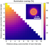 |
Fig. 7 Depiction of the overlap ratio |


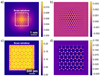 |
Fig. 8 (a) Real and (b) imaginary parts of the transmission function |


3.2.2 Comparison to the focused-probe case
Projected potential measurements by WDD and SBI-D, expressed in V⋅nm, are displayed in Figure 10, for the specified values of  , alongside the corresponding square roots of Fourier transform amplitude. Similarly to the conventional focused-probe case, specimen frequencies are already detected at
  , although a clear observation of real-space features in the scan window is, arguably, only possible for
  . One further qualitative observation can be made on the noise in the micrographs, which seems more persistent than in those shown in Section 2.1. This is expected, since the use of a delocalized illumination implies an equivalent spread of retrievable information per recording, as explained in the previous paragraph.
Another important difference between the overfocused and the conventional cases is a slight loss of resolution, e.g. consistent with comparisons made in reference [147]. As the true aberration function of the illumination was included in the process, and since the number of single recordings and camera pixelisation were high enough, this cannot be attributed to an insufficiency of available scattering information [145,202] or a processing error. In particular, increasing the number of scan positions to 32 by 32 did not improve the resolution, hence showing no further need in overlap ratio. Another explanation can be found in the inherent information content of the acquired MR-STEM dataset, as determined by the CRLB [195,196]. In other words, different illumination conditions, including probe focus [196], may possess specific capacities to transfer specimen frequencies to the acquired data, hence leading to a supplementary  -dependent weighting in the result. In that context, ptychographic reconstructions, with their practical resolution limits, can be expected to remain probe-specific, even when this probe is known or refined in-process [69,70,107,148].
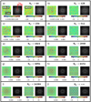 |
Fig. 9 Results of analytical ptychography of monolayer MoS2, applied on the multislice electron diffraction simulation presented in Section 2.2. Calculations are done for a variety of average numbers of electrons per pattern |


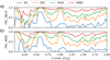 |
Fig. 10 FRC calculated from the |


3.2.3 Fourier ring correlations
Moreover, Fourier ring correlations FRCm(k) were calculated for the overfocused probe case and are displayed in Figures 10a for SBI-D and 10b for WDD. They show essentially the same features as were observed in Figure 5, in particular with four peaks at coordinates k corresponding to specimen frequencies. A difference is however found in the apparently lower dose-efficiency, which can be attributed to the wider illuminated area, as explained above. Noteworthily, this effect is likely amplified by the larger amount of pixels per frequency ranges Rk, which is due to the greater size of the reconstruction window, leading to a more important weighting of frequency coordinates without crystal lattice information. This is particularly visible when comparing the first and second peaks to the third and fourth ones.
3.2.4 Phase shift value range
Going back to the micrographs themselves, a few more remarks can be made on the ranges of value covered by the projected potential maps. First, in the case of the WDD result, a similar, though slightly smaller, range is obtained as in the focused-probe case. In that context, the reduction can be related to the loss of resolution, and thus to less strongly peaked atomic sites. The average potential in the scan window is also greater. This should nevertheless serve to highlight that the retrieved DC component, i.e. the mean phase shift in the reconstruction window, is arbitrary and only depends, numerically, on the size of the reconstruction window and on the sampling of specimen features, including beyond the scanned area.
The SBI-D result, on the other hand, shows a drastically lower range of values in comparison to Figure 4, nearly four orders of magnitude down. Interestingly, whereas  is unaffected by this problem, as mentioned above, it is not the case for the transmission function itself. To understand this, an important difference between the two analytical ptychography methods should be highlighted again, which is that WDD measures the projected potential in an indirect manner, i.e. by extracting the angle of the initially retrieved
  , post-use of equation (14). As such, it is determined by the ratio between its real and imaginary parts, irrespective of the amplitude. A comparison of the
  map obtained in the conventional focused-probe case, as shown in Figures 8c and 8d, to the one retrieved in the overfocused case, in Figures 8a and 8b, is sufficient to confirm the role of this indirect measurement process in avoiding a similar defocus-induced value range issue as met for the SBI-D calculation. In particular, in the overfocused case, the amplitude of the measured transmission function is found to possess values more than an order of magnitude smaller than the focused-probe reconstructions, similarly to the SBI-D case though not as strongly, while the ratio of real and imaginary parts remains roughly the same.
As a supplementary note here, the slice-wise transmission functions actually used for the simulation, one set for each frozen phonon configuration, are all phase objects in the strict sense, i.e. with a constant unitary amplitude. This reflects the absence of absorption effects for the interacting electrons, which is assumed to be fully elastic. The measurement by ptychography, on the other hand, should in general not be expected to fulfill this condition, as mentioned in Section 2.1.
3.3 Role of the numerical aperture
3.3.1 Simulation and processing parameters
In analytical ptychography, the range of accessible frequencies is, outside of super-resolution [74,98,143–146], determined strictly by qA = sin(α)/λ. In this subsection, an interest is thus taken in how the numerical aperture sin(α) affects the dose requirement of the reconstruction. Consequently, two supplementary simulations were performed given α = 15 mrad, in a scan grid of 32 by 32 points, and α = 60 mrad, with 128 by 128 scan points. For reference, the resulting unaberrated probes possess Rayleigh criterions δrRayleigh of 198 and 49 pm, respectively. Other than that, simulation parameters were identical as those described in Section 2.1.
Under those illumination conditions, the relation  , with Ns the total number of scan positions, is fulfilled, which leads to approximately the same
  values in all tested focused-probe cases, including in Section 2.1. The accessible frequency range is however twice smaller in the 15 mrad case, and twice larger in the 60 mrad one. Moreover, for both cases, the same selection of
  values was used as for the conventional focused-probe case, hence leading to comparable count sparsity in the exploited CBED patterns. The resulting doses nevertheless differ due to the change in the number of scan points.
Here, it should furthermore be noted that, for most instruments, using a semi-convergence angle of 60 mrad is either not technically possible or leads to an excessive loss of coherence due to chromatic aberration [203]. In this publication, the use of such large numerical aperture should thus be regarded as relevant for theoretical verification rather than an immediate experimental horizon, although some work has already been performed in that direction within the last few years [204–207].
3.3.2 Noise level in the micrographs
The results of applying the iCoM, SBI-D and WDD methods to the 15 mrad simulation are displayed in Figure 11, and those of the 60 mrad simulation in Figure 12. Owing to the different values of α, the indicated qA differs among the two cases. An immediate consequence of the reduced frequency surface, for the 15 mrad case, is a resolution insufficient to clearly separate two neighboring atomic sites. As such, in Figure 11, the crystal lattice is visible only thanks to its hexagonal structure, i.e. the cavity in the middle of an given hexagon can be resolved, and no more than half of the first order of lattice-induced frequencies is transferred. In comparison, for the 30 mrad simulation presented in Sections 2.1 and 2.2, two orders, i.e. four hexagonal patterns of frequency peaks, were visible in the Fourier transform. Under α = 60 mrad, the resolution is significantly improved, and up to 11 hexagons can be seen.
Continuing, for both new values of α, the specimen frequencies are visible in the Fourier transform, even with excessive noise in real-space, already from the lowest doses introduced. Beyond this, as  increases, the observed level of noise and relative strength of specimen frequencies evolve in a rather similar manner among the three focused-probe cases tested in this section, including Figure 4, with the reconstruction being nearly noiseless at
  . The same method-dependent frequency transfer capacities are furthermore observed in each case, in particular with an important presence of low-frequency artefacts in the iCoM result and slightly more persistent high-frequency noise in the WDD micrograph than for SBI, as explained previously.
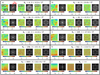 |
Fig. 11 Results of analytical ptychography of monolayer MoS2, applied on the multislice electron diffraction simulation presented in Section 2.3, given α = 15 mrad. Calculations are done for a variety of average numbers of electrons per pattern |


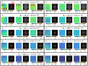 |
Fig. 12 Results of analytical ptychography of monolayer MoS2, applied on the multislice electron diffraction simulation presented in Section 2.3, given α = 60 mrad. Calculations are done for a variety of average numbers of electrons per pattern |


3.3.3 Fourier ring correlations
Those first qualitative remarks are confirmed by the calculated Fourier ring correlations, shown in Figure 13 for the 15 mrad case and in Figure 14 for the 60 mrad one. The general behaviour described in Section 2.1 is observed for the two newly introduced numerical apertures too. In particular, the  -dependent dose-efficiency is higher for
  -coordinates that are rich in specimen information and lower for the others, where noise reduction is only due to the normalization. Moreover, as is particularly visible in Figure 14, the manner in which FRCm (k) is calculated for each method leads to an artificially lower dose-efficiency for higher k, owing to the more important weighting of noisy
  -coordinates in the corresponding Rk range. It should finally be noted that the micrographs shown in Figures 11 and 12 confirm findings from Section 2.1 relating to the value range of the retrieved phase shift maps. Specifically, the WDD range is about twice as high as the SBI-D and iCoM ones. Beyond that, the resolution, in leading to more or less pronounced atomic peaks, contributes as well to this effect.
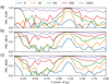 |
Fig. 13 FRC calculated from the |


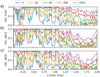 |
Fig. 14 FRC calculated from the |


3.3.4 Dose requirement and reconstructed frequencies
At a fundamental level, the results presented in this subsection confirm, as was noted by equation (30), that the overall dose requirement of a ptychographic reconstruction, to obtain a specific precision determined by CRLBRS, is proportional to qA2 and more generally to the surface covered by the reconstructed two-dimensional frequency space. This is expected, as a larger frequency surface implies a larger number of pixels to which Poisson noise [150] is propagated from the detector plane.
From a naive standpoint, as long as a well-focused probe is employed and that  is fulfilled, thus permitting the conservation of the same area overlap, this notion also implies that the relation between the average number of electrons per pattern
  and the noise level is not fundamentally dependent on the numerical aperture. In other words, it can be expected that, irrespective of the resolution, reconstruction can be performed with very low
  , and thus with sparse CBED patterns [105], the dose being then fixed by the number of scan points. As such, count sparsity in itself is not a limitation for the reconstruction of the electrostatic potential by analytical ptychography. Noteworthily, if the other common strategy is adopted, consisting in recording in the defocused geometry [117,118],
  will need to be increased to match the information content of the focused-probe data. A revised area overlap is then also necessary, as shown in Section 2.2.
4 Imaging of apoferritin particles under high- and low-resolution conditions
4.1 Contrast predictions above vacuum
4.1.1 Difficulties in imaging light matter
In Section 2, interest was taken in the atomically resolved measurement of the projected potential in a monolayer 2D material which, though it often requires an acceleration voltage U below e.g. 80 kV to avoid excessive knock-on displacement of atoms [208,209], remains an experimentally realistic endeavour. On the other hand, the critical dose [25] of many beam-sensitive specimens, e.g. biological matter, is in practice too low to permit high-resolution imaging, unless done through the combination of a large number of images from identical objects, i.e. a single-particle analysis (SPA) [210,211] procedure. In particular, the dose requirement is proportional to the surface of reconstructed frequencies, as was exemplified in Section 2.3. Consequently, electron ptychography performed on viruses and proteins [1,61–64] has so far been focused on retrieving relatively small ranges of frequency components and limited resolutions.
It should also be noted that the amount of electrons needed depends on the imaged specimen itself. Specifically, it depends on the encountered atom types and their scattering cross-section [212,213], which determines the general amount of observed specimen-induced features in the scattering patterns. In other words, the heavier the imaged material is, the stronger the contrast ends up being in the retrieved phase shift map. This factor, as well as the high probability of radiolysis [27,214,215] leading to the dose limitations mentioned above, make biological specimens particularly difficult to investigate in STEM.
4.1.2 Simulation and processing parameters
In order to explore this topic further and, like in the MoS2 case, empirically determine the dose requirement for the imaging of a macromolecule in the absence of further issues, e.g. the MTF of the camera, scan imperfections or an amorphous ice embedding, new simulations were performed based on an apoferritin particle in vacuum. The chosen acceleration voltage U was 300 keV. Two distinct semi-convergence angles α were furthermore tested, specifically 1.5 and 6.0 mrad, to verify the previously observed trends on the role of the numerical aperture. In both cases, a field of view of 15 nm by 15 nm, with the specimen in the center, was employed. This field of view was filled by 642 scan positions in the 1.5 mrad simulation, and by 2562 positions in the 6.0 mrad one.
Importantly, those illumination conditions both permit an area overlap  slightly above 82%, when comparing immediately neighboring scan points, and lead to Rayleigh criteria δrRayleigh of about 801 and 200 pm, respectively. Moreover, following a suggestion made e.g. in reference [151,216], the probe focus was placed in the middle of the vertical distance covered by the specimen. Given the large depths of focus δzDOF = λ/(2sin(α/2)2) [121,122] of about 1750 nm, for α = 1.5 mrad, and 109 nm, for 6.0 mrad, this is nevertheless not expected to be critical here. In particular, and also because such a light material is not expected to lead to e.g. strong channeling effects [123], the wave amplitude should remain sufficiently invariant throughout the propagation axis so that the POA can be considered fulfilled in any case.
Like in the previous section, the multislice method [181–183] was used to represent the elastic propagation of the electron wavefunction through matter, while the atomic potentials were parameterized according to reference [184]. As before, the specimen potential was pixelated in the two-dimensional plane such that a maximum scattering vector of up to twice the range actually used could be simulated. The object was furthermore sliced in the manner described in reference [110]. To perform the calculations in a reasonable time, owing to the large size of the simulation window, thermal vibrations were accounted for by multiplying the scattering amplitudes with an isotropic Debye–Waller factor, i.e. the wave was considered to interact coherently with a time-average of the atoms in motion. In general, this approximation may lead to errors for high enough scattering angles [133], e.g. above 40 to 50 mrad, but was not considered to be problematic here, as the extent of  -space available was below this limit.
The results of applying reconstructions on the 1.5 mrad simulation are presented in Figure 15, and those of the 6.0 mrad one in Figure 16. Dose-limitation was imposed based on the procedure described in Appendix B, while employing average numbers of electron per pattern  equal to 2
l
, with l ∈ [2, 3, ..., 10]. The resulting doses are indicated in the figures. For all cases, both the measured projected potential map, expressed in V⋅nm, and the square root of its Fourier transform amplitude are displayed. For all cases, the single CBED patterns were normalized to their sum pre-treatment and the SFPA solution, described in Section 2.5 was employed for practical implementation.
equal to 2
l
, with l ∈ [2, 3, ..., 10]. The resulting doses are indicated in the figures. For all cases, both the measured projected potential map, expressed in V⋅nm, and the square root of its Fourier transform amplitude are displayed. For all cases, the single CBED patterns were normalized to their sum pre-treatment and the SFPA solution, described in Section 2.5 was employed for practical implementation.
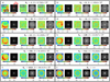 |
Fig. 15 Results of analytical ptychography of apoferritin, applied on the multislice electron diffraction simulation presented in Section 3.1, with α = 1.5 mrad. Calculations are done for a variety of average numbers of electrons per pattern |


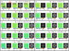 |
Fig. 16 Results of analytical ptychography of apoferritin, applied on the multislice electron diffraction simulation presented in Section 3.1, with α = 6.0 mrad. Calculations are done for a variety of average numbers of electrons per pattern |


4.1.3 Noise level and contrast transfer
As a first remark, specimen frequencies are not as obviously observable in the Fourier transforms as in the MoS2 case. In particular, there are no lattice-induced frequency peaks with a width dependent on the size of the scan window to be observed, but rather a complex specimen pattern corresponding to this specific projection of the potential. The overall shape of the particle is also easy to notice in real-space, e.g. from  . This is especially true in the iCoM result, where the higher weighting of low-frequencies, high-frequency information having then been reduced, permits an easy detection of the edges [173,172]. This is nevertheless accompanied by a prevalence of low-frequency noise, as explained in the previous section. For the other imaging modes, the two distinct numerical apertures used permit the visibility of a varying degree of details in the inner structure of the specimen.
Furthermore, the CTF  , for SBI, and
  , for iCoM, lead to clear differences between the different micrographs, as those two methods highlight specific information in the projected potential map. In contrast, in the case of an atomically resolved crystal where specimen frequencies are sparse, as mentioned above, those effects are not as striking. Upon comparing the two analytical ptychography approaches, it can thus be noticed that the presence of
  leads to an exaggeration of the intermediary frequencies, e.g. close to
  , as is especially visible in the high-dose micrographs.
Relating to arguments given in the MoS2 case, as well as in Section 2.3, such a clear difference between the SBI-D and WDD results indicates that the imaged specimen cannot be strictly defined as a weak scatterer, i.e.  does not intrinsically apply while, under the WPOA, it should represent the information content of the scattering data itself and thus occur in all ptychographic imaging modes. This is furthermore confirmed by the value ranges of the WDD phase shift maps themselves, which are found above 0.4 rad for α = 1.5 mrad and 0.7 rad for α = 6.0 mrad, at infinite dose. Such a finding is of particular interest here, as it demonstrates that considering biological specimens as weak phase objects, even with a low value of σ following equation (2), may not be correct in the general case.
Outside of those aspects, the  -dependent measurement precision is found to be comparable among the two qA cases, as explained in Section 2.3. This thus implies, following the necessary adaptation of Ns for the conservation of the area overlap, a proportionality between the required dose and the frequency surface being reconstructed, which here extends to qA2 directly as was illustrated by equation (30). The count sparsity of the CBED patterns used is furthermore not a limitation for the reconstruction itself, as expected from previous results. While
  increases, internal features of the particle become better resolved, thus here providing a direct empirical verification of the dose requirement of specifically targeted structural information.
4.1.4 Fourier ring correlations
Those observations are confirmed by the calculated FRCm(k), as shown in Figure 17, for the 1.5 mrad case, and in Figure 18, for the 6.0 mrad one. Like in Section 2, no striking differences of dose-efficiency are observed among the three imaging modes used in this work, which again is reflective of the comparable needed dose to reach the best achievable precision for a given frequency component. This furthermore illustrate the preponderant role of the CTF in making high- and low-frequency noise more persistent in the WDD and iCoM micrographs, respectively.
As was highlighted previously as well, the FRC shows much more difficulty in reaching high dose-dependent precision for higher frequencies k in general, which can be related to the higher number of pixels in the corresponding Rk range. Moreover, the absence of frequency peaks, owing to the difference of structure in the Fourier transform, observed in the previous paragraph, can be noted here as well and leads to a more homogeneous variation of the FRC, though a specific frequency response is still visible. Relating to Figures 15 and 16, it is noteworthy that this specific frequency response, upon comparing the dose-limited cases to the infinite dose reconstruction, can arguably be noticed from e.g.  .
.
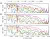 |
Fig. 17 FRC calculated from the |


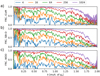 |
Fig. 18 FRC calculated from the |


4.1.5 Phase shift value range
Finally, going back to the micrographs themselves, it should be noted that the different imaging modes, much like for the MoS2 simulations, do not lead to the same general value ranges, though this time the effect depends on the semi-convergence angle α as well. This confirms the hypothesis made in Section 2.1 that disagreements in the range of values covered by the retrieved phase shift map, outside of the role of the resolution and of the reconstructed frequency surface, are related to the methods themselves.
4.2 Influence of protective amorphous ice
4.2.1 Simulation and processing parameters
While Section 4.1 was sufficient to provide a general prospect for the imaging of biological objects via analytical ptychography, it left out an important practical aspect of such experiments. When performing TEM imaging on this type of specimens, it is common to first embed them in a relatively thick layer of amorphous ice, in order to permit stability in a vacuum environment [214]. This experimental protocol is known for leading to a so-called structural noise [217] effect in the result. In particular, as the micrograph should represent a vertical projection of the illuminated object [218], the frequency distribution of the ice directly adds up to the image spectrum, potentially creating difficulties of interpretation.
In order to investigate this effect further in the case of analytical ptychography, the simulations described in Section 4.1 were repeated with a specimen consisting of the same apoferritin particle, though this time embedded within a representative amorphous ice layer. The ice and particle ensemble, having a total thickness of about 50 nm, was relaxed via molecular dynamics, as described in reference [110], before performing the actual multislice calculation. The focus point of the probe was placed in the middle of the object, and other simulation parameters were chosen identically to the in-vacuum simulation cases.
4.2.2 Noise level and contrast transfer
Results of applying the imaging methods to the new simulations are displayed in Figure 19, for α = 1.5 mrad, and in Figure 20, for 6.0 mrad. In general, the remarks made in Section 4.1 can be transferred to this second situation as well. In particular, the visualization of the overall specimen structure in real-space is possible from about  and the CTF of iCoM and SBI lead to very different final images among the methods. The main difference is the presence of the projected potential of the ice, superposed to the contribution of the apoferritin particle and thus leading to the deterministic noise-like effect [217] mentioned in the last paragraph.
An important difference in its overall influence should furthermore be noted between the two semi-convergence angles employed here. Specifically, while the 1.5 mrad case does not show a very striking loss of contrast due to the ice, as can be observed by comparing it to Figure 15, the 6.0 mrad one is affected much more strongly. In particular, in the SBI-D and WDD images, the particle is nearly not visible at all anymore, in contrast to Figure 16 where its inner structure was well-resolved even at relatively low doses.
As can be directly noticed in the Fourier transforms, the frequency spectrum of the amorphous ice, which possesses a ring-like shape owing to its amorphous structure [218,219], is added to the specimen frequencies, thus obstructing them in the resulting image. It is then clear that, while the value of 1.5 mrad is sufficiently small to mostly cut off the affected  -coordinates, then found beyond the 2qA limit, it is not so in the 6.0 mrad case. In this context, due to its large thickness compared to the apoferritin itself, the amorphous ice furthermore ends up dominating the projected potential measurement, and thus preventing a direct interpretation of the micrograph. Noteworthily, the iCoM method, in Figure 20 is the least affected of the three, which is related to its CTF attenuating higher frequency components.
In general, those findings show that, for the imaging of a single ice-embedded biological object, not only does the frequency distribution of the amorphous ice has to be known beforehand [218], but the numerical aperture may need to be adapted as well in order to obtain an interpretable micrograph. That is, unless further post-processing is employed like in the context of SPA [210,211]. It is moreover clear that, if the WPOA does not strictly apply to a protein particle standing in vacuum, it will be the case as well for its ice-embedded version.
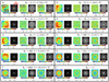 |
Fig. 19 Results of analytical ptychography of apoferritin, applied on the multislice electron diffraction simulation presented in Section 3.2, with α = 1.5 mrad. Calculations are done for a variety of average numbers of electrons per pattern |


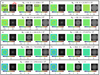 |
Fig. 20 Results of analytical ptychography of apoferritin, applied on the multislice electron diffraction simulation presented in Section 3.2, with α = 6.0 mrad. Calculations are done for a variety of average numbers of electrons per pattern |


4.2.3 Fourier ring correlations
For completeness of the arguments, FRC calculations were performed for both cases and are displayed in Figures 21 and 22, respectively for 1.5 and 6.0 mrad. As expected, the results displayed in Figure 21 do not show obvious differences from those in Figure 17, while the FRC profiles in Figure 22 have completely changed from their in-vacuum version, as displayed in Figure 18. Specifically, at the coordinates k where the ice-induced ring of frequencies is highest, the fine structure of specimen-related information has been largely replaced by a near-homogeneous response.
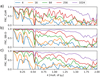 |
Fig. 21 FRC calculated from the |


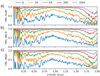 |
Fig. 22 FRC calculated from the |


5 Discussion
5.1 Comparison of frequency transfer capacities and role of the interaction model
5.1.1 Generalizable contrast transfer function for a weak scatterer
The three STEM-based phase retrieval techniques used in this work, encompassing the iCoM approach and the two existing analytical ptychography methods, can be distinguished in how well they recover specimen information at reconstructible spatial frequencies  . In particular, they may be attributed contrast transfer functions, denoting a
  -dependent attenuation of signal-to-noise ratio. In principle, such frequency-wise reductions of the object spectrum can be solved by deconvolving the result with the predicted point-spread function. This is however difficult in the low-dose case, as the concerned
  -coordinates may then have been brought below the noise level, hence resulting in significant noise amplification upon deconvolution. As a result, the dose-efficiency is then expected to be much worse for frequency components where the CTF has a low value.
A first step towards determining the CTF is the derivation of the intrinsic phase contrast transfer function  [104], depicted in Figure 1, occurring when the illuminated specimen is a weak phase object and being then reflective of a sideband-like geometry in the acquired scattering data. Owing to this geometry, the SBI method [103,104] constitutes an optimized approach for the reconstruction of the phase shift map, where parts of the data containing only noise are excluded as explained in Section 2.3.
More generally, when the WPOA is fulfilled, the PCTF  is applicable to all methods investigated in this work, which implies the equality of the WDD and SBI results, given a high enough dose. The known form of the PCTF, and the resulting
  -dependent noise level in SBI [149], furthermore make it possible to establish a noise normalization strategy [106,149], rendering the noise level homogeneous across the full frequency spectrum of the retrieved object.
In the particular case of iCoM imaging, and as explained in Section 2.4, a supplementary frequency weighting is imposed, following the optical transfer function  [114,168] shown in Figure 2. In contrast to the PCTF arising in the case of a weak scatterer, this OTF is due to the much simpler measurement method based on the prior calculation of the average momentum transfer at each scan position, and does not represent the information content of the experiment. As such, under the WPOA, both
  and
and  can be expected to apply to the iCoM result.
5.1.2 Specimen-dependent frequency transfer
Continuing, from the results presented in this work, it should nevertheless be clear that the WPOA is inappropriate in the general case. Specifically, it was shown, for both the monolayer MoS2 and the apoferritin model-objects, that not only did the SBI and WDD results differed in a clear manner, but also that the retrieved ranges of phase shift exceeded those of weak scatterers. What this then implies is the inapplicability of the derived  as a general PCTF in focused-probe ptychography. In this context, it is noteworthy that, due to its process still being based on the assumption of a weak phase object, the SBI method may then remove useful specimen information from the available scattering data rather than just noise, and still imposes
  as a CTF [106,151].
This is not the case of the WDD method, which only assumes the more general POA, and consists in a complete deconvolution of the four-dimensional Wigner distribution  of the illumination from the scattering data. As such, and in contrast to iCoM and SBI, its process may be expected to lead to no supplementary
  -wise reduction in signal-to-noise ratio, at least outside of the frequency-dependent CRLB [195,196], then representing the fundamental information content of the data.
At a deeper level, what this means is that, while the WPOA allowed for the extraction of a specimen-independent frequency transfer capacity in ptychography, the POA alone does not permit this simplification. This then implies that the empirical CTF of the WDD method should always be expected to depend on the illuminated specimen and its scattering power [193,194]. In general, more work on the CRLB as a theoretical precision metric will be needed in the future, as it can be used to derive inhomogeneities along  -space, for different specific cases. Noteworthily, this encompasses the role of the aberration function which, even when included in the process, still affects the reconstruction [196], as exemplified in Section 2.2.
5.1.3 Further limitations
Continuing on the WDD method, the absence of a truly process-induced frequency attenuation effect may remain true only as long as the assumed interaction model, i.e. the fully coherent POA, is fulfilled. In this condition, equation (12) is correct and may be used as an accurate basis for the treatment of the scattering data. A first practical limit is the partial coherence of the illumination, which imposes an envelope effect in  [112].
Furthermore, in the case where the specimen is too thick to be accurately described as a phase object, but a ptychographic reconstruction is still performed on the basis of a single transmission function, artificial features may then be introduced in the result [108,151,220]. In this context, it is also noteworthy that, even with a thicker specimen, using an optimally focused illumination has been shown to partly alleviate the artificial features mentioned above [151,216], as is also well-known in the case of CoM and DPC [163–167]. In iterative ptychography, another increasingly popular solution is the inclusion of a multislice propagation within the process [221–224], i.e. the use of a more accurate interaction model.
5.1.4 Use of dark field electrons and super-resolution
One more advantage of the WDD method, in comparison to SBI, is its ability to exploit the dark field electrons, which are otherwise neglected under the WPOA, as shown by equations (17) and (20).
Importantly, in focused-probe ptychography, the use of the scattering vectors above qA is also necessary to achieve super-resolution [74,98,143–146], i.e. the ability to enhance resolution in real-space by accessing spatial frequencies that extend beyond the diffraction limit. The spectrum of the object is then completed outside of the conventional 2qA range, by exploiting the relation of the intensity scattered outside the primary beam with those initially missing frequencies. In practice, for analytical ptychography, this is done through the stepping out approach [98,113].
Because of its ability for super-resolution, WDD has the potential to access much larger frequency ranges than SBI and iCoM, though this requires a significant amount of electrons to be present in the dark field, which makes this approach very expensive in terms of dose [147]. As the present work focuses on the imaging of beam-sensitive specimens, that topic was left out of it.
5.2 Other aspects of the reconstruction strategy for low-dose imaging
5.2.1 Dose requirement
Overarchingly, this publication verifies that the dose requirement of ptychography is proportional to the frequency surface to be reconstructed. In the case where no super-resolution [74,98,143–146] is sought, this proportionality extends directly to qA2.
As illustrated by equation (30), this furthermore implies that the total number of detected electrons, needed to reach a certain accuracy in the real-space measurement, should be expected to be proportional to the quantity of reconstructed frequency pixels  . What this then means is that, in general, to achieve a pre-defined signal-to-noise ratio in the micrograph, the numerical aperture has to be adapted to the critical dose of the imaged specimen [25,199].
Furthermore, while super-resolution may be of interest for many other applications, it should realistically not be relied on for the low-dose imaging of beam-sensitive objects, as it is based on exploiting the least intense scattering vectors across the far-field. Consequently, enhancing the resolution when imaging such specimens should rather be done by enlarging the numerical aperture itself, as this then represents the least dose-expensive option.
5.2.2 Normalization
An appropriate normalization choice is also important in analytical ptychography, especially in the case where the acquired data is sparse [105], and thus where large changes in the variance of single patterns occur across the scan window. For this purpose, the strategy proposed in reference [149], consisting in dividing the acquisitions by their individual sums pre-treatment, was adopted in this work.
Noteworthily, this pattern-wise approach is equivalent to performing the calculation while adapting the normalization of the electron wavefunction itself to the number of counts in each corresponding pattern. Further investigations on the normalization strategy may otherwise be relevant in the future, which will also need to be correctly accounted for in any estimation of the theoretical measurement precision, e.g. using the CRLB [198].
5.2.3 Use of a Wiener filter
Finally, in the case of the WDD and SBI-D processes, the use of a Wiener filter [139] as a deconvolution method implies the introduction of a parameter ϵ to avoid divisions by zero, as included in equations (13) and (19). Whereas, at infinite dose, this number may be considered as a simple numerical precision term, it in practice needs to be adapted to the noise level in the distributions  and
and  to avoid its amplification in the final result. This is however at the cost of accuracy for the reconstruction itself, i.e. the range of phase shift values and the transfer of higher frequencies are affected, as noted in more details e.g. in reference [225].
In this work, a single ϵ = 10−6 was consistently used in all deconvolutions, which was found sufficient to avoid noise amplification, including in the condition of highest count sparsity, or an unwanted modification of the value range in the retrieved phase shift maps, as verified in the infinite dose case.
High values of ϵ, up to 10−3, were tested as well in the WDD reconstruction, with no further reductions in the noise level, but leading to excessive modifications of the result in high-dose conditions. In the case of SBI, comparisons were performed between the deconvolutive form, using the Wiener parameter of 10−6, and the summative form. This was done for the few lowest doses considered and did not show a better signal-to-noise ratio in the SBI-S result, hence confirming the stability of the deconvolutive process in this case. There too, higher values did not permit an improved noise level compared to the 10−6 case. For both the WDD and SBI-D processes, ϵ = 10−7 furthermore led to a slight, but clear, amplification of the noise.
Importantly, the stability of both the WDD and SBI-D calculations, even with very sparse scattering data and given no adaptation of the parameter to the dose, can be related in large part to the scan position-wise normalization strategy chosen here. In particular, it ensures that each treated CBED pattern has a total value of one, hence leading to a reduction in their individual variances [149]. As such, similar value ranges are consistently found in the amplitudes of the distributions  and
and  . Other practical choices included the use of orthonormal Fourier transforms. In this context, the precise selection of the Wiener parameter ϵ becomes less critical for the reconstruction, which then permits more reproducible performances for the analytical ptychography procedures.
As a final note on this topic, reaching a correspondence between the ranges of phase shift covered by the SBI and the WDD results, which was an argument used in reference [225], should not be an objective in choosing a value for the Wiener parameter ϵ. As was extensively discussed in Section 4.1 and noted e.g. in reference [108], the two methods are generally expected to lead to different results, since their fundamental assumptions on the specimen differ. On the other hand, once ϵ has been elevated sufficiently above zero to make sure that numerical divergence and noise amplification are avoided even with very sparse data, there is little justification in further increasing it. In fact, the higher this parameter becomes, the farther away the numerical operation goes from an actual inversion, and the less representative of the real interaction the deconvolved Wigner distribution  becomes. As such, the change in values for the retrieved WDD phase shift, induced by an increment of ϵ, should be seen as artefactual rather than a possible validation of the SSB/SBI result.
6 Conclusion
Analytical ptychography methods present several advantages for the imaging of beam-sensitive materials. Specifically, they are direct, fast and relatively easy to implement. Their requirements in terms of computer memory can furthermore be reduced to allow efficient parallelization and GPU implementation, for instance through the scan-frequency partitioning algorithm introduced in this publication. They also do not require a specific choice in reconstruction parameters for particular cases, such as e.g. a coupling of loss and regularization functions, the batch size or an update strength, which could otherwise be needed to obtain a satisfying output. Finally, they permit the treatment of sparse scattering data [105] with no risk of numerical divergence.
Overall, those advantages make analytical ptychography especially relevant for the low-dose investigation of beam-sensitive objects, where the same measurement often has to be repeated multiple times to reach an accurate result, thus creating a need for streamlined acquisition and reconstruction procedures, even encompassing live processing [100,101]. In that manner, the direct form of analytical ptychography would also facilitate the inclusion in a more complex experimental protocol, such as e.g. three-dimensional structure retrieval based on a single-particle analysis [62,210,211]. Moreover, in this context, potential reproducibility issues could be prevented, given the uniqueness of the processing compared to the high variability among iterative algorithms and their parameter sets.
Acknowledgments
The authors acknowledge financial support from the Horizon 2020 research and innovation programme, as well as from the European Research Council within the Horizon Europe innovation funding programme.
Funding
H.L.L.R. and J.V. acknowledge funding from the Horizon 2020 research and innovation programme (European Union), under grant agreement No 101017720 (FET-Proactive EBEAM). M.L.L. and K.M.-C. acknowledge funding from the European Research Council within the Horizon Europe innovation funding programme under Grant Agreement 101118656 (ERC Synergy project 4D-BioSTEM).
Conflicts of interest
The authors declare no conflicts of interest.
Data availability statement
No experimental data was required in this publication.
Author contribution statement
H.L.L.R.: conceptualization, methodology, software, simulation, data treatment, writing. M.L.L.: simulation, draft review. K.M.-C.: draft review, supervision. J.V.: conceptualization, draft review, supervision.
References
- L. Zhou, J. Song, J.S. Kim, X. Pei, C. Huang, M. Boyce, L. Mendonça, D. Clare, A. Siebert, C.S. Allen, E. Liberti, D. Stuart, X. Pan, P.D. Nellist, P. Zhang, A.I. Kirkland, P. Wang, Low-dose phase retrieval of biological specimens using cryo-electron ptychography, Nat. Commun. 11, 2773 (2020). https://doi.org/10.1038/s41467-020-16391-6 [Google Scholar]
- I. Lazić, M. Wirix, M.L. Leidl, F. de Haas, D. Mann, M. Beckers, E.V. Pechnikova, K. Müller-Caspary, R. Egoavil, E.G. Bosch, C. Sachse, Single-particle cryo-EM structures from iDPC-STEM at near-atomic resolution, Nat. Methods 19, 1126 (2022). https://doi.org/10.1038/s41592-022-01586-0 [Google Scholar]
- K. Müller-Caspary, M. Duchamp, M. Rösner, V. Migunov, F. Winkler, H. Yang, M. Huth, R. Ritz, M. Simson, S. Ihle, H. Soltau, T. Wehling, R.E. Dunin-Borkowski, S. Van Aert, A. Rosenauer, Atomic-scale quantification of charge densities in two-dimensional materials, Phys. Rev. B 98 (2018). https://doi.org/10.1103/PhysRevB.98.121408 [Google Scholar]
- Y. Wen, C. Ophus, C.S. Allen, S. Fang, J. Chen, E. Kaxiras, A.I. Kirkland, J.H. Warner, Simultaneous identification of low and high atomic number atoms in monolayer 2D materials using 4D scanning transmission electron microscopy, Nano Lett. 19, 6482 (2019). https://doi.org/10.1021/acs.nanolett.9b02717 [Google Scholar]
- Y. Chen, T.-C. Chou, C.-H. Fang, C.-Y. Lu, C.-N. Hsiao, W.-T. Hsu, C.-C. Chen, Direct observation of single-atom defects in monolayer two-dimensional materials by using electron ptychography at 200 kV acceleration voltage, Sci. Rep. 14, 277 (2024). https://doi.org/10.1038/s41598-023-50784-z [Google Scholar]
- L. Liu, N. Wang, C. Zhu, X. Liu, Y. Zhu, P. Guo, L. Alfilfil, X. Dong, D. Zhang, Y. Han, Direct imaging of atomically dispersed molybdenum that enables location of aluminum in the framework of zeolite ZSM-5, Angew. Chem. In. Ed. 59, 819 (2020). https://doi.org/10.1002/anie.201909834 [Google Scholar]
- H. Sha, J. Cui, J. Li, Y. Zhang, W. Yang, Y. Li, R. Yu, Ptychographic measurements of varying size and shape along zeolite channels, Sci. Adv. 9, 1 (2023). https://doi.org/10.1126/sciadv.adf1151 [Google Scholar]
- H. Zhang, G. Li, J. Zhang, D. Zhang, Z. Chen, X. Liu, P. Guo, Y. Zhu, C. Chen, L. Liu, X. Guo, Y. Han, Three-dimensional inhomogeneity of zeolite structure and composition revealed by electron ptychography, Science 380, 633 (2023). https://doi.org/10.1126/science.adg3183 [Google Scholar]
- Z. Dong, E. Zhang, Y. Jiang, Q. Zhang, A. Mayoral, H. Jiang, Y. Ma, Atomic-level imaging of zeolite local structures using electron ptychography, J. Am. Chem. Soc. 145, 6628 (2023). https://doi.org/10.1021/jacs.2c12673 [Google Scholar]
- K. Mitsuishi, K. Nakazawa, R. Sagawa, M. Shimizu, H. Matsumoto, H. Shima, T. Takewaki, Direct observation of Cu in high-silica chabazite zeolite by electron ptychography using Wigner distribution deconvolution, Sci. Rep. 13, 316 (2023). https://doi.org/10.1038/s41598-023-27452-3 [CrossRef] [Google Scholar]
- J.G. Lozano, G.T. Martinez, L. Jin, P.D. Nellist, P.G. Bruce, Low-dose aberration-free imaging of li-rich cathode materials at various states of charge using electron ptychography, Nano Lett. 18, 6850 (2018). https://doi.org/10.1021/acs.nanolett.8b02718 [Google Scholar]
- W. Song, M.A. Pérez-Osorio, J.-J. Marie, E. Liberti, X. Luo, C. O'Leary, R.A. House, P.G. Bruce, P.D. Nellist, Direct imaging of oxygen shifts associated with the oxygen redox of Li-rich layered oxides, Joule 6, 1049 (2022). https://doi.org/10.1016/j.joule.2022.04.008 [Google Scholar]
- W. Song, M.A. Pérez-Osorio, J. Chen, Z. Ding, J.-J. Marie, M. Juelsholt, R.A. House, P.G. Bruce, P.D. Nellist, Visualization of Tetrahedral Li in the Alkali Layers of Li-Rich Layered Metal Oxides, J. Am. Chem. Soc. 146, 23814 (2024). https://doi.org/10.1021/jacs.4c05556 [Google Scholar]
- B. Hao, Z. Ding, X. Tao, P.D. Nellist, H.E. Assender, Atomic-scale imaging of polyvinyl alcohol crystallinity using electron ptychography, Polymer 284, 126305 (2023). https://doi.org/10.1016/j.polymer.2023.126305 [Google Scholar]
- M. Ma, X. Zhang, X. Chen, H. Xiong, L. Xu, T. Cheng, J. Yuan, F. Wei, B. Shen, In situ imaging of the atomic phase transition dynamics in metal halide perovskites, Nat. Commun. 14, 7142 (2023). https://doi.org/10.1038/s41467-023-42999-5 [Google Scholar]
- A. Scheid, Y. Wang, M. Jung, T. Heil, D. Moia, J. Maier, P.A. van Aken, Electron ptychographic phase imaging of beam-sensitive all-inorganic halide perovskites using four-dimensional scanning transmission electron microscopy, Microsc. Microanal. 29, 869 (2023). https://doi.org/10.1093/micmic/ozad017 [Google Scholar]
- N.J. Schrenker, T. Braeckevelt, A. De Backer, N. Livakas, C.-P. Yu, T. Friedrich, M.B.J. Roeffaers, J. Hofkens, J. Verbeeck, L. Manna, V. Van Speybroeck, S. Van Aert, S. Bals, Investigation of the octahedral network structure in formamidinium lead bromide nanocrystals by low-dose scanning transmission electron microscopy, Nano Lett. 24, 10936 (2024). https://doi.org/10.1021/acs.nanolett.4c02811 [Google Scholar]
- X. Li, J. Wang, X. Liu, L. Liu, D. Cha, X. Zheng, A.A. Yousef, K. Song, Y. Zhu, D. Zhang, Y. Han, Direct imaging of tunable crystal surface structures of mof mil-101 using high-resolution electron microscopy, J. Am. Chem. Soc. 141, 12021 (2019). https://doi.org/10.1021/jacs.9b04896 [Google Scholar]
- G. Li, M. Xu, W.-q. Tang, Y. Liu, C. Chen, D. Zhang, L. Liu, S. Ning, H. Zhang, Z.-y. Gu, Z. Lai, D.A. Muller, Y. Han, Atomically resolved imaging of radiation-sensitive metal-organic frameworks via electron ptychography, Nat. Commun. 16, 914 (2025). https://doi.org/10.1038/s41467-025-56215-z [Google Scholar]
- R. Egerton, Radiation damage to organic and inorganic specimens in the TEM, Micron 119, 72 (2019). https://doi.org/10.1016/j.micron.2019.01.005 [Google Scholar]
- W.E. King, R. Benedek, K. Merkle, M. Meshii, Damage effects of high energy electrons on metals, Ultramicroscopy 23, 345 (1987). https://doi.org/10.1016/0304-3991(87)90245-2 [Google Scholar]
- L.W. Hobbs, F.W. Clinard, S.J. Zinkle, R.C. Ewing, Radiation effects in ceramics, J. Nucl. Mater. 216, 291 (1994). https://doi.org/10.1016/0022-3115(94)90017-5 [Google Scholar]
- B. Bornes, W. Glaser, Über die Temperaturerhöhung der Objekte im Übermikroskop, Kolloid-Z. 106, 123 (1944). https://doi.org/10.1007/BF01502110 [Google Scholar]
- D.T. Grubb, Radiation damage and electron microscopy of organic polymers, J. Mater. Sci. 9, 1715 (1974). https://doi.org/10.1007/BF00540772 [Google Scholar]
- R.F. Egerton, Dose measurement in the TEM and STEM, Ultramicroscopy 229, 113363 (2021). https://doi.org/10.1016/j.ultramic.2021.113363 [Google Scholar]
- R. Egerton, Limits to the spatial, energy and momentum resolution of electron energy-loss spectroscopy, Ultramicroscopy 107, 575 (2007). https://doi.org/10.1016/j.ultramic.2006.11.005 [CrossRef] [PubMed] [Google Scholar]
- P. Rez, Coherent and incoherent imaging of biological specimens with electrons and X-rays, Ultramicroscopy 231, 113301 (2021). https://doi.org/10.1016/j.ultramic.2021.113301 [Google Scholar]
- G. McMullan, D. Cattermole, S. Chen, R. Henderson, X. Llopart, C. Summerfield, L. Tlustos, A. Faruqi, Electron imaging with Medipix2 hybrid pixel detector, Ultramicroscopy 107, 401 (2007). https://doi.org/10.1016/j.ultramic.2006.10.005 [Google Scholar]
- X. Llopart, R. Ballabriga, M. Campbell, L. Tlustos, W. Wong, Timepix, a 65k programmable pixel readout chip for arrival time, energy and/or photon counting measurements, Nucl. Instrum. Methods Phys. Res. A 581, 485 (2007). https://doi.org/10.1016/j.nima.2007.08.079 [Google Scholar]
- R. Ballabriga, M. Campbell, E. Heijne, X. Llopart, L. Tlustos, W. Wong, Medipix3: A 64k pixel detector readout chip working in single photon counting mode with improved spectrometric performance, Nucl. Instrum. Methods Phys. Res. A 633, S15 (2011). https://doi.org/10.1016/j.nima.2010.06.108 [Google Scholar]
- R. Plackett, I. Horswell, E.N. Gimenez, J. Marchal, D. Omar, N. Tartoni, Merlin: a fast versatile readout system for Medipix3, JINST 8, C01038 (2013). https://doi.org/10.1088/1748-0221/8/01/C01038 [Google Scholar]
- T. Poikela, J. Plosila, T. Westerlund, M. Campbell, M.D. Gaspari, X. Llopart, V. Gromov, R. Kluit, M.V. Beuzekom, F. Zappon, V. Zivkovic, C. Brezina, K. Desch, Y. Fu, A. Kruth, Timepix3: a 65K channel hybrid pixel readout chip with simultaneous ToA/ToT and sparse readout, JINST 9, C05013 (2014). https://doi.org/10.1088/1748-0221/9/05/C05013 [CrossRef] [Google Scholar]
- H. Ryll, M. Simson, R. Hartmann, P. Holl, M. Huth, S. Ihle, Y. Kondo, P. Kotula, A. Liebel, K. Müller-Caspary, A. Rosenauer, R. Sagawa, J. Schmidt, H. Soltau, L. Strüder, A pnCCD-based, fast direct single electron imaging camera for TEM and STEM, JINST 11, P04006 (2016). https://doi.org/10.1088/1748-0221/11/04/P04006 [Google Scholar]
- M.W. Tate, P. Purohit, D. Chamberlain, K.X. Nguyen, R. Hovden, C.S. Chang, P. Deb, E. Turgut, J.T. Heron, D.G. Schlom, D.C. Ralph, G.D. Fuchs, K.S. Shanks, H.T. Philipp, D.A. Muller, S.M. Gruner, High dynamic range pixel array detector for scanning transmission electron microscopy, Microsc. Microanal. 22, 237 (2016). https://doi.org/10.1017/S1431927615015664 [CrossRef] [PubMed] [Google Scholar]
- H.T. Philipp, M.W. Tate, K.S. Shanks, L. Mele, M. Peemen, P. Dona, R. Hartong, G. van Veen, Y.-T. Shao, Z. Chen, J. Thom-Levy, D.A. Muller, S.M. Gruner, Very-high dynamic range, 10,000 frames/second pixel array detector for electron microscopy, Microsc. Microanal. 28, 425 (2022). https://doi.org/10.1017/S1431927622000174 [Google Scholar]
- X. Llopart, J. Alozy, R. Ballabriga, M. Campbell, R. Casanova, V. Gromov, E. Heijne, T. Poikela, E. Santin, V. Sriskaran, L. Tlustos, A. Vitkovskiy, Timepix4, a large area pixel detector readout chip which can be tiled on 4 sides providing sub-200 ps timestamp binning, JINST 17, C01044 (2022). https://doi.org/10.1088/1748-0221/17/01/C01044 [Google Scholar]
- P. Zambon, S. Bottinelli, R. Schnyder, D. Musarra, D. Boye, A. Dudina, N. Lehmann, S. De Carlo, M. Rissi, C. Schulze-Briese, M. Meffert, M. Campanini, R. Erni, L. Piazza, KITE: High frame rate, high count rate pixelated electron counting ASIC for 4D STEM applications featuring high-Z sensor, Nucl. Instrum. Methods Phys. Res. A 1048, 167888 (2023). https://doi.org/10.1016/j.nima.2022.167888 [Google Scholar]
- P. Ercius, I.J. Johnson, P. Pelz, B.H. Savitzky, L. Hughes, H.G. Brown, S.E. Zeltmann, S.-L. Hsu, C.C.S. Pedroso, B.E. Cohen, R. Ramesh, D. Paul, J.M. Joseph, T. Stezelberger, C. Czarnik, M. Lent, E. Fong, J. Ciston, M.C. Scott, C. Ophus, A.M. Minor, P. Denes, The 4D Camera: An 87 kHz direct electron detector for scanning/transmission electron microscopy, Microsc. Microanal. 30, 903 (2024) https://doi.org/10.1093/mam/ozae086 [Google Scholar]
- R.S. Ruskin, Z. Yu, N. Grigorieff, Quantitative characterization of electron detectors for transmission electron microscopy, J. Struct. Biol. 184, 385 (2013). https://doi.org/10.1016/j.jsb.2013.10.016 [Google Scholar]
- A.-C. Milazzo, G. Moldovan, J. Lanman, L. Jin, J.C. Bouwer, S. Klienfelder, S.T. Peltier, M.H. Ellisman, A.I. Kirkland, N.-H. Xuong, Characterization of a direct detection device imaging camera for transmission electron microscopy, Ultramicroscopy 110, 741 (2010). https://doi.org/10.1016/j.ultramic.2010.03.007 [Google Scholar]
- J.A. Mir, R. Clough, R. MacInnes, C. Gough, R. Plackett, I. Shipsey, H. Sawada, I. MacLaren, R. Ballabriga, D. Maneuski, V. O'Shea, D. McGrouther, A.I. Kirkland, Characterisation of the Medipix3 detector for 60 and 80 keV electrons, Ultramicroscopy 182, 44 (2017). https://doi.org/10.1016/j.ultramic.2017.06.010 [CrossRef] [PubMed] [Google Scholar]
- K.A. Paton, M.C. Veale, X. Mu, C.S. Allen, D. Maneuski, C. Kübel, V. O'Shea, A.I. Kirkland, D. McGrouther, Quantifying the performance of a hybrid pixel detector with GaAs:Cr sensor for transmission electron microscopy, Ultramicroscopy 227, 113298 (2021). https://doi.org/10.1016/j.ultramic.2021.113298 [Google Scholar]
- K. Müller, H. Ryll, I. Ordavo, S. Ihle, L. Strüder, K. Volz, J. Zweck, H. Soltau, A. Rosenauer, Scanning transmission electron microscopy strain measurement from millisecond frames of a direct electron charge coupled device, Appl. Phys. Lett. 101, 212110 (2012). https://doi.org/10.1063/1.4767655 [Google Scholar]
- K. Müller-Caspary, F.F. Krause, F. Winkler, A. Béché, J. Verbeeck, S. Van Aert, A. Rosenauer, S. VanAert, A. Rosenauer, Comparison of first moment STEM with conventional differential phase contrast and the dependence on electron dose, Ultramicroscopy 203, 95 (2018) in print. https://doi.org/10.1016/j.ultramic.2018.12.018 [Google Scholar]
- H. Yang, L. Jones, H. Ryll, M. Simson, H. Soltau, Y. Kondo, R. Sagawa, H. Banba, I. MacLaren, P.D. Nellist, 4D STEM: High efficiency phase contrast imaging using a fast pixelated detector, J. Phys.: Conf. Ser. 644, 12032 (2015). https://doi.org/10.1088/1742-6596/644/1/012032 [Google Scholar]
- G. Fan, P. Datte, E. Beuville, J.-F. Beche, J. Millaud, K. Downing, F. Burkard, M. Ellisman, N.-H. Xuong, ASIC-based event-driven 2D digital electron counter for TEM imaging, Ultramicroscopy 70, 107 (1998). https://doi.org/10.1016/S0304-3991(97)00109-5 [Google Scholar]
- E. Frojdh, M. Campbell, M.D. Gaspari, S. Kulis, X. Llopart, T. Poikela, L. Tlustos, Timepix3: first measurements and characterization of a hybrid-pixel detector working in event driven mode, JINST 10, C01039 (2015). https://doi.org/10.1088/1748-0221/10/01/C01039 [Google Scholar]
- D. Jannis, C. Hofer, C. Gao, X. Xie, A. Béché, T. Pennycook, J. Verbeeck, Event driven 4D STEM acquisition with a Timepix3 detector: Microsecond dwell time and faster scans for high precision and low dose applications, Ultramicroscopy 233, 113423 (2022). https://doi.org/10.1016/j.ultramic.2021.113423 [CrossRef] [PubMed] [Google Scholar]
- Y. Auad, J. Baaboura, J.D. Blazit, M. Tencé, O. Stéphan, M. Kociak, L.H. Tizei, Time calibration studies for the Timepix3 hybrid pixel detector in electron microscopy, Ultramicroscopy 257, 113889 (2024). https://doi.org/10.1016/j.ultramic.2023.113889 [Google Scholar]
- J. Kuttruff, J. Holder, Y. Meng, P. Baum, Real-time electron clustering in an event-driven hybrid pixel detector, Ultramicroscopy 255, 113864 (2024). https://doi.org/10.1016/j.ultramic.2023.113864 [Google Scholar]
- W. Hoppe, Beugung im inhomogenen Primärstrahlwellenfeld. I. Prinzip einer Phasenmessung von Elektronenbeungungsinterferenzen, Acta Crystallogr. A 25, 495 (1969). https://doi.org/10.1107/S0567739469001045 [Google Scholar]
- W. Hoppe, G. Strube, Beugung in inhomogenen Primärstrahlenwellenfeld. II. Lichtoptische Analogieversuche zur Phasenmessung von Gitterinterferenzen, Acta Crystallogr. A 25, 502 (1969). https://doi.org/10.1107/S0567739469001057 [Google Scholar]
- W. Hoppe, Beugung im inhomogenen Primärstrahlwellenfeld. III. Amplituden- und Phasenbestimmung bei unperiodischen Objekten, Acta Crystallogr. A 25, 508 (1969). https://doi.org/10.1107/S0567739469001069 [Google Scholar]
- A. Drenth, A. Huiser, H. Ferwerda, The problem of phase retrieval in light and electron microscopy of strong objects, Optica Acta 22, 615 (1975). https://doi.org/10.1080/713819083 [Google Scholar]
- J.R. Fienup, Reconstruction of an object from the modulus of its Fourier transform, Opt. Lett. 3, 27 (1978). https://doi.org/10.1364/OL.3.000027 [NASA ADS] [CrossRef] [Google Scholar]
- J. Miao, D. Sayre, H.N. Chapman, Phase retrieval from the magnitude of the Fourier transforms of nonperiodic objects, J. Opt. Soc. Am. A 15, 1662 (1998). https://doi.org/10.1364/JOSAA.15.001662 [NASA ADS] [CrossRef] [Google Scholar]
- J. Miao, P. Charalambous, J. Kirz, D. Sayre, Extending the methodology of X-ray crystallography to allow imaging of micrometre-sized non-crystalline specimens, Nature 400, 342 (1999). https://doi.org/10.1038/22498 [Google Scholar]
- U. Weierstall, Q. Chen, J. Spence, M. Howells, M. Isaacson, R. Panepucci, Image reconstruction from electron and X-ray diffraction patterns using iterative algorithms: experiment and simulation, Ultramicroscopy 90, 171 (2002). https://doi.org/10.1016/S0304-3991(01)00134-6 [Google Scholar]
- G.J. Williams, H.M. Quiney, B.B. Dhal, C.Q. Tran, K.A. Nugent, A.G. Peele, D. Paterson, M.D. de Jonge, Fresnel coherent diffractive imaging, Phys. Rev. Lett. 97, 025506 (2006). https://doi.org/10.1103/PhysRevLett.97.025506 [Google Scholar]
- J.R. Fienup, Phase retrieval algorithms: a comparison, Appl. Opt. 21, 2758 (1982). https://doi.org/10.1364/AO.21.002758 [NASA ADS] [CrossRef] [Google Scholar]
- P.M. Pelz, W.X. Qiu, R. Bücker, G. Kassier, R.J. Miller, Low-dose cryo electron ptychography via non-convex Bayesian optimization, Sci. Rep. 7, 1 (2017). https://doi.org/10.1038/s41598-017-07488-y [CrossRef] [Google Scholar]
- X. Pei, L. Zhou, C. Huang, M. Boyce, J.S. Kim, E. Liberti, Y. Hu, T. Sasaki, P.D. Nellist, P. Zhang, D.I. Stuart, A.I. Kirkland, P. Wang, Cryogenic electron ptychographic single particle analysis with wide bandwidth information transfer, Nat. Commun. 14, 3027 (2023). https://doi.org/10.1038/s41467-023-38268-0 [Google Scholar]
- B. Küçükoğlu, I. Mohammed, R.C. Guerrero-Ferreira, S.M. Ribet, G. Varnavides, M.L. Leidl, K. Lau, S. Nazarov, A. Myasnikov, M. Kube, J. Radecke, C. Sachse, K. Müller-Caspary, C. Ophus, H. Stahlberg, Low-dose cryo-electron ptychography of proteins at sub-nanometer resolution, Nat. Commun. 15, 8062 (2024). https://doi.org/10.1038/s41467-024-52403-5 [Google Scholar]
- W. Mao, W. Zhang, C. Huang, L. Zhou, J.S. Kim, S. Gao, Y. Lei, X. Wu, Y. Hu, X. Pei, W. Fang, X. Liu, J. Song, C. Fan, Y. Nie, A.I. Kirkland, P. Wang, Multi-Convergence-Angle Ptychography with Simultaneous Strong Contrast and High Resolution (2024) arXiv:2403.16902. https://doi.org/10.48550/arXiv.2403.16902 [Google Scholar]
- V. Elser, Phase retrieval by iterated projections, J. Opt. Soc. Am. A 20, 40 (2003). https://doi.org/10.1364/JOSAA.20.000040 [Google Scholar]
- H.M. Faulkner, J.M. Rodenburg, Movable aperture lensless transmission microscopy: A novel phase retrieval algorithm, Phys. Rev. Lett. 93, 2 (2004). https://doi.org/10.1103/PhysRevLett.93.023903 [Google Scholar]
- J.M. Rodenburg, H.M. Faulkner, A phase retrieval algorithm for shifting illumination, Appl. Phys. Lett. 85, 4795 (2004). https://doi.org/10.1063/1.1823034 [Google Scholar]
- P. Thibault, M. Dierolf, A. Menzel, O. Bunk, C. David, F. Pfeiffer, High-resolution scanning X-ray diffraction microscopy, Science 321, 379 (2008). https://doi.org/10.1126/science.1158573 [Google Scholar]
- P. Thibault, M. Dierolf, O. Bunk, A. Menzel, F. Pfeiffer, Probe retrieval in ptychographic coherent diffractive imaging, Ultramicroscopy 109, 338 (2009). https://doi.org/10.1016/j.ultramic.2008.12.011 [Google Scholar]
- A.M. Maiden, J.M. Rodenburg, An improved ptychographical phase retrieval algorithm for diffractive imaging, Ultramicroscopy 109, 1256 (2009). https://doi.org/10.1016/j.ultramic.2009.05.012 [CrossRef] [PubMed] [Google Scholar]
- A. Maiden, D. Johnson, P. Li, Further improvements to the ptychographical iterative engine, Optica 4, 736 (2017). https://doi.org/10.1364/optica.4.000736 [Google Scholar]
- A. Maiden, W. Mei, P. Li, WASP: Weighted Average of Sequential Projections for ptychographic phase retrieval, Optics Express 32, 21327 (2024). https://doi.org/10.1364/oe.516946 [Google Scholar]
- R. Gerchberg, W. Saxton, Optik 35, 237 (1972). http://ci.nii.ac.jp/naid/10010556614/ [Google Scholar]
- R. Gerchberg, Super-resolution through error energy reduction, Optica Acta 21, 709 (1974). https://doi.org/10.1080/713818946 [Google Scholar]
- M. Guizar-Sicairos, J.R. Fienup, Phase retrieval with transverse translation diversity: a nonlinear optimization approach, Opt. Express 16, 7264 (2008). https://doi.org/10.1364/oe.16.007264 [Google Scholar]
- P. Godard, M. Allain, V. Chamard, J. Rodenburg, Noise models for low counting rate coherent diffraction imaging, Opt. Express 20, 25914 (2012). https://doi.org/10.1364/OE.20.025914 [Google Scholar]
- L. Bian, J. Suo, J. Chung, X. Ou, C. Yang, F. Chen, Q. Dai, Fourier ptychographic reconstruction using Poisson maximum likelihood and truncated Wirtinger gradient, Sci. Rep. 6, 1 (2016). https://doi.org/10.1038/srep27384 [CrossRef] [Google Scholar]
- M. Odstrčil, A. Menzel, M. Guizar-Sicairos, Iterative least-squares solver for generalized maximum-likelihood ptychography, Opt. Express 26, 3108 (2018). https://doi.org/10.1364/oe.26.003108 [Google Scholar]
- P. Thibault, M. Guizar-Sicairos, Maximum-likelihood refinement for coherent diffractive imaging, New J. Phys. 14, 1 (2012). https://doi.org/10.1088/1367-2630/14/6/063004 [Google Scholar]
- M. Pham, P. Yin, A. Rana, S. Osher, J. Miao, Generalized proximal smoothing (GPS) for phase retrieval, Opt. Express 27, 2792 (2019). https://doi.org/10.1364/OE.27.002792 [Google Scholar]
- M. Schloz, T.C. Pekin, Z. Chen, W. Van den Broek, D.A. Muller, C.T. Koch, Overcoming information reduced data and experimentally uncertain parameters in ptychography with regularized optimization, Opt. Express 28, 28306 (2020). https://doi.org/10.1364/oe.396925 [Google Scholar]
- K.C. Lee, H. Chae, S. Xu, K. Lee, R. Horstmeyer, S.A. Lee, B.-W. Hong, Anisotropic regularization for sparsely sampled and noise-robust Fourier ptychography, Opt. Express 32, 25343 (2024). https://doi.org/10.1364/OE.529023 [Google Scholar]
- Z. Herdegen, B. Diederichs, K. Müller-Caspary, Thermal vibrations in the inversion of dynamical electron scattering, Phys. Rev. B 110, 064102 (2024). https://doi.org/10.1103/PhysRevB.110.064102 [Google Scholar]
- B. Diederichs, Z. Herdegen, A. Strauch, F. Filbir, K. Müller-Caspary, Exact inversion of partially coherent dynamical electron scattering for picometric structure retrieval, Nat. Commun. 15 (2024). https://doi.org/10.1038/s41467-023-44268-x [Google Scholar]
- W. Yang, H. Sha, J. Cui, L. Mao, R. Yu, Local-orbital ptychography for ultrahigh-resolution imaging, Nat. Nanotechnol. 19, 612 (2024). https://doi.org/10.1038/s41565-023-01595-w [Google Scholar]
- W. Yang, H. Sha, J. Cui, R. Yu, Imaging thick objects with deep-sub-angstrom resolution and deep-sub-picometer precision (2025) arXiv:2502.18294. https://doi.org/10.48550/arXiv.2502.18294 [Google Scholar]
- H. Chang, P. Enfedaque, J. Zhang, J. Reinhardt, B. Enders, Y.-S. Yu, D. Shapiro, C.G. Schroer, T. Zeng, S. Marchesini, Advanced denoising for X-ray ptychography, Opt. Express 27, 10395 (2019). https://doi.org/10.1364/OE.27.010395 [Google Scholar]
- M.L. Leidl, B. Diederichs, C. Sachse, K. Müller-Caspary, Influence of loss function and electron dose on ptychography of 2D materials using the Wirtinger flow, Micron 185, 103688 (2024). https://doi.org/10.1016/j.micron.2024.103688 [Google Scholar]
- J. Seifert, Y. Shao, R. van Dam, D. Bouchet, T. van Leeuwen, A.P. Mosk, Maximum-likelihood estimation in ptychography in the presence of Poisson-Gaussian noise statistics, Opt. Lett. 48, 6027 (2023). https://doi.org/10.1364/OL.502344 [Google Scholar]
- O. Melnyk, Convergence properties of gradient methods for blind ptychography (2023) arXiv:2306.08750. https://doi.org/10.48550/arXiv.2306.08750 [Google Scholar]
- V. Katkovnik, J. Astola, Sparse ptychographical coherent diffractive imaging from noisy measurements, J. Optical Soc. Am. A 30, 367 (2013). https://doi.org/10.1364/JOSAA.30.000367 [Google Scholar]
- S. Marchesini, H. Krishnan, B.J. Daurer, D.A. Shapiro, T. Perciano, J.A. Sethian, F.R. Maia, SHARP: a distributed GPU-based ptychographic solver, J. Appl. Crystallogr. 49, 1245 (2016). https://doi.org/10.1107/S1600576716008074 [Google Scholar]
- X. Yu, V. Nikitin, D.J. Ching, S. Aslan, D. Gürsoy, T. Biçer, Scalable and accurate multi-GPU-based image reconstruction of large-scale ptychography data, Sci. Rep. 12, 1 (2022). https://doi.org/10.1038/s41598-022-09430-3 [CrossRef] [Google Scholar]
- X. Wang, A. Tsaris, D. Mukherjee, M. Wahib, P. Chen, M. Oxley, O. Ovchinnikova, J. Hinkle, Image gradient decomposition for parallel and memory-efficient ptychographic reconstruction, in SC22: International Conference for High Performance Computing, Networking, Storage and Analysis (IEEE, 2022) Vol. 2022-Novem, pp. 1–13. arXiv:2205.06327. https://doi.org/10.1109/SC41404.2022.00013 [Google Scholar]
- D. Mukherjee, K.M. Roccapriore, A. Al-Najjar, A. Ghosh, J.D. Hinkle, A.R. Lupini, R.K. Vasudevan, S.V. Kalinin, O.S. Ovchinnikova, M.A. Ziatdinov, N.S. Rao, A roadmap for edge computing enabled automated multidimensional transmission electron microscopy, Microscopy Today 30, 10 (2022). https://doi.org/10.1017/S1551929522001286 [Google Scholar]
- S.S. Welborn, C. Harris, S.M. Ribet, G. Varnavides, C. Ophus, B. Enders, P. Ercius, Streaming large-scale microscopy data to a supercomputing facility (2024) arXiv:2407.03215. https://doi.org/10.48550/arXiv.2407.03215 [Google Scholar]
- R. Bates, J. Rodenburg, Sub-ångström transmission microscopy: A fourier transform algorithm for microdiffraction plane intensity information, Ultramicroscopy 31, 303 (1989). https://doi.org/10.1016/0304-3991(89)90052-1 [Google Scholar]
- J.M. Rodenburg, R.H.T. Bates, The theory of super-resolution electron microscopy via Wigner-distribution deconvolution, Philos. Trans. R. Soc. Lond. A 339, 521 (1992). https://doi.org/10.1098/rsta.1992.0050 [Google Scholar]
- J. Rodenburg, B. McCallum, P. Nellist, Experimental tests on double-resolution coherent imaging via STEM, Ultramicroscopy 48, 304 (1993). https://doi.org/10.1016/0304-3991(93)90105-7 [CrossRef] [Google Scholar]
- A. Strauch, D. Weber, A. Clausen, A. Lesnichaia, A. Bangun, B. März, F.J. Lyu, Q. Chen, A. Rosenauer, R. Dunin-Borkowski, K. Müller-Caspary, Live processing of momentum-resolved STEM data for first moment imaging and ptychography, Microsc. Microanal. 27, 1078 (2021). https://doi.org/10.1017/S1431927621012423 [Google Scholar]
- A. Bangun, P.F. Baumeister, A. Clausen, D. Weber, R.E. Dunin-Borkowski, Wigner distribution deconvolution adaptation for live ptychography reconstruction, Microsc. Microanal. 29, 994 (2023). https://doi.org/10.1093/micmic/ozad021 [Google Scholar]
- D. Weber, S. Ehrig, A. Schropp, A. Clausen, S. Achilles, N. Hoffmann, M. Bussmann, R.E. Dunin-Borkowski, C.G. Schroer, Live Iterative Ptychography, Microsc. Microanal. 30, 103 (2024). https://doi.org/10.1093/mam/ozae004 [Google Scholar]
- T.J. Pennycook, A.R. Lupini, H. Yang, M.F. Murfitt, L. Jones, P.D. Nellist, Efficient phase contrast imaging in STEM using a pixelated detector. Part 1: Experimental demonstration at atomic resolution, Ultramicroscopy 151, 160 (2015). https://doi.org/10.1016/j.ultramic.2014.09.013 [CrossRef] [PubMed] [Google Scholar]
- H. Yang, T.J. Pennycook, P.D. Nellist, Efficient phase contrast imaging in STEM using a pixelated detector. Part II: Optimisation of imaging conditions, Ultramicroscopy 151, 232 (2015). https://doi.org/10.1016/j.ultramic.2014.10.013 [Google Scholar]
- C.M. O'Leary, C.S. Allen, C. Huang, J.S. Kim, E. Liberti, P.D. Nellist, A.I. Kirkland, Phase reconstruction using fast binary 4D STEM data, Appl. Phys. Lett. 116, 124101 (2020). https://doi.org/10.1063/1.5143213 [Google Scholar]
- C.M. O'Leary, G.T. Martinez, E. Liberti, M.J. Humphry, A.I. Kirkland, P.D. Nellist, Contrast transfer and noise considerations in focused-probe electron ptychography, Ultramicroscopy 221, 113189 (2021). https://doi.org/10.1016/j.ultramic.2020.113189 [CrossRef] [PubMed] [Google Scholar]
- H. Yang, R.N. Rutte, L. Jones, M. Simson, R. Sagawa, H. Ryll, M. Huth, T.J. Pennycook, M.L.H. Green, H. Soltau, Y. Kondo, B.G. Davis, P.D. Nellist, Simultaneous atomic-resolution electron ptychography and Z-contrast imaging of light and heavy elements in complex nanostructures, Nat. Commun. 7, 1 (2016). https://doi.org/10.1038/ncomms12532 [CrossRef] [Google Scholar]
- H. Yang, I. MacLaren, L. Jones, G.T. Martinez, M. Simson, M. Huth, H. Ryll, H. Soltau, R. Sagawa, Y. Kondo, C. Ophus, P. Ercius, L. Jin, A. Kovács, P.D. Nellist, Electron ptychographic phase imaging of light elements in crystalline materials using Wigner distribution deconvolution, Ultramicroscopy 180, 173 (2017). https://doi.org/10.1016/j.ultramic.2017.02.006 [Google Scholar]
- P. Wang, F. Zhang, S. Gao, M. Zhang, A.I. Kirkland, Electron ptychographic diffractive imaging of boron atoms in LaB 6 crystals, Sci. Rep. 7, 1 (2017). https://doi.org/10.1038/s41598-017-02778-x [CrossRef] [Google Scholar]
- M.L. Leidl, C. Sachse, K. Müller-Caspary, Dynamical scattering in ice-embedded proteins in conventional and scanning transmission electron microscopy, IUCrJ 10, 867 (2023). https://doi.org/10.1107/S2052252523004505 [Google Scholar]
- B. McCallum, J. Rodenburg, Two-dimensional demonstration of Wigner phase-retrieval microscopy in the STEM configuration, Ultramicroscopy 45, 371 (1992). https://doi.org/10.1016/0304-3991(92)90149-E [Google Scholar]
- P. Nellist, J. Rodenburg, Beyond the conventional information limit: the relevant coherence function, Ultramicroscopy 54, 61 (1994). https://doi.org/10.1016/0304-3991(94)90092-2 [Google Scholar]
- P. Li, T.B. Edo, J.M. Rodenburg, Ptychographic inversion via Wigner distribution deconvolution: noise suppression and probe design, Ultramicroscopy 147, 106 (2014). https://doi.org/10.1016/j.ultramic.2014.07.004 [Google Scholar]
- K. Müller, F.F. Krause, A. Béché, M. Schowalter, V. Galioit, S. Löffler, J. Verbeeck, J. Zweck, P. Schattschneider, A. Rosenauer, Atomic electric fields revealed by a quantum mechanical approach to electron picodiffraction, Nat. Commun. 5, 5653 (2014). https://doi.org/10.1038/ncomms6653 [Google Scholar]
- I. Lazić, E.G.T. Bosch, S. Lazar, Phase contrast {STEM} for thin samples: Integrated differential phase contrast, Ultramicroscopy 160, 265 (2016). https://doi.org/10.1016/j.ultramic.2015.10.011 [CrossRef] [PubMed] [Google Scholar]
- H. Yang, P. Ercius, P.D. Nellist, C. Ophus, Enhanced phase contrast transfer using ptychography combined with a pre-specimen phase plate in a scanning transmission electron microscope, Ultramicroscopy 171, 117 (2016). https://doi.org/10.1016/j.ultramic.2016.09.002 [Google Scholar]
- F. Hüe, J.M. Rodenburg, A.M. Maiden, F. Sweeney, P.A. Midgley, Wave-front phase retrieval in transmission electron microscopy via ptychography, Phys. Rev. B 82, 1 (2010). https://doi.org/10.1103/PhysRevB.82.121415 [CrossRef] [Google Scholar]
- J. Song, C.S. Allen, S. Gao, C. Huang, H. Sawada, X. Pan, J. Warner, P. Wang, A.I. Kirkland, Atomic resolution defocused electron ptychography at low dose with a fast, direct electron detector, Sci. Rep. 9, 3919 (2019). https://doi.org/10.1038/s41598-019-40413-z [Google Scholar]
- D.J. Vine, G.J. Williams, B. Abbey, M.A. Pfeifer, J.N. Clark, M.D. de Jonge, I. McNulty, A.G. Peele, K.A. Nugent, Ptychographic Fresnel coherent diffractive imaging, Phys. Rev. A 80, 063823 (2009). https://doi.org/10.1103/PhysRevA.80.063823 [Google Scholar]
- J.M. Cowley, I. Sumio, S. Iijima, Electron microscope image contrast for thin crystal, Z. Naturforsch. A 27, 445 (1972). https://doi.org/10.1515/zna-1972-0312 [Google Scholar]
- K. van Benthem, A.R. Lupini, M. Kim, H.S. Baik, S. Doh, J.-H. Lee, M.P. Oxley, S.D. Findlay, L.J. Allen, J.T. Luck, S.J. Pennycook, Three-dimensional imaging of individual hafnium atoms inside a semiconductor device, Appl. Phys. Lett. 87, 034104 (2005). https://doi.org/10.1063/1.1991989 [Google Scholar]
- K. van Benthem, A.R. Lupini, M.P. Oxley, S.D. Findlay, L.J. Allen, S.J. Pennycook, Three-dimensional ADF imaging of individual atoms by through-focal series scanning transmission electron microscopy, Ultramicroscopy 106, 1062 (2006). https://doi.org/10.1016/j.ultramic.2006.04.020 [Google Scholar]
- D. Van Dyck, M. Op de Beeck, A simple intuitive theory for electron diffraction, Ultramicroscopy 64, 99 (1996). https://doi.org/10.1016/0304-3991(96)00008-3 [Google Scholar]
- C.J. Humphreys, P.B. Hirsch, Absorption parameters in electron diffraction theory, Philos. Mag. 18, 115 (1968). https://doi.org/10.1080/14786436808227313 [Google Scholar]
- H. Yoshioka, Effect of inelastic waves on electron diffraction, J. Phys. Soc. Jpn. 12, 618 (1957). https://doi.org/10.1143/JPSJ.12.618 [Google Scholar]
- Z.L. Wang, W.D. Mo, The “ Optical potential ” and multiple diffuse scattering in dynamical electron diffraction and imaging, Scanning Microsc. 12, 91 (1998) [Google Scholar]
- K.A. Mkhoyan, S.E. MacCagnano-Zacher, M.G. Thomas, J. Silcox, Critical role of inelastic interactions in quantitative electron microscopy, Phys. Rev. Lett. 100, 1 (2008). https://doi.org/10.1103/PhysRevLett.100.025503 [Google Scholar]
- A. Beyer, F.F. Krause, H.L. Robert, S. Firoozabadi, T. Grieb, P. Kükelhan, D. Heimes, M. Schowalter, K. Müller-Caspary, A. Rosenauer, K. Volz, Influence of plasmon excitations on atomic-resolution quantitative 4D scanning transmission electron microscopy, Sci. Rep. 10, 17890 (2020). https://doi.org/10.1038/s41598-020-74434-w [Google Scholar]
- J. Barthel, M. Cattaneo, B.G. Mendis, S.D. Findlay, L.J. Allen, Angular dependence of fast-electron scattering from materials, Phys. Rev. B 101, 1 (2020). https://doi.org/10.1103/PhysRevB.101.184109 [Google Scholar]
- H.L. Robert, B. Diederichs, K. Müller-Caspary, Contribution of multiple plasmon scattering in low-angle electron diffraction investigated by energy-filtered atomically resolved 4D-STEM, Appl. Phys. Lett. 121, 213502 (2022). https://doi.org/10.1063/5.0129692 [Google Scholar]
- C.R. Hall, The scattering of high energy electrons by the thermal vibrations of crystals, Philos. Mag. 12, 815 (1965). https://doi.org/10.1080/14786436508218919 [Google Scholar]
- C.R. Hall, P.B. Hirsch, Effect of thermal diffuse scattering on propagation of high energy electrons through crystals, Proc. R. Soc. Lond. A 286, 158 (1965). https://doi.org/10.1098/rspa.1965.0136 [Google Scholar]
- D. Van Dyck, Is the frozen phonon model adequate to describe inelastic phonon scattering? Ultramicroscopy 109, 677 (2009). https://doi.org/10.1016/j.ultramic.2009.01.001 [Google Scholar]
- K. Fujiwara, Relativistic dynamical theory of electron diffraction, J. Phys. Soc. Jpn. 16, 2226 (1961). https://doi.org/10.1143/JPSJ.16.2226 [Google Scholar]
- O. Bunk, M. Dierolf, S. Kynde, I. Johnson, O. Marti, F. Pfeiffer, Influence of the overlap parameter on the convergence of the ptychographical iterative engine, Ultramicroscopy 108, 481 (2008). https://doi.org/10.1016/j.ultramic.2007.08.003 [Google Scholar]
- J.M. Cowley, Image contrast in a transmission scanning electron microscope, Appl. Phys. Lett. 15, 58 (1969). https://doi.org/10.1063/1.1652901 [Google Scholar]
- F.F. Krause, A. Rosenauer, Reciprocity relations in transmission electron microscopy: a rigorous derivation, Micron 92, 1 (2017). https://doi.org/10.1016/j.micron.2016.09.007 [Google Scholar]
- E. Wigner, On the quantum correction for thermodynamic equilibrium, Phys. Rev. 40, 749 (1932). https://doi.org/10.1103/PhysRev.40.749 [CrossRef] [Google Scholar]
- R.T. Bates, M.J. McDonnell, Image restoration and reconstruction (Oxford University Press, Inc., 1986) [Google Scholar]
- G. Möllenstedt, H. Düker, Fresnelscher Interferenzversuch mit einem Biprisma für Elektronenwellen, Naturwissenschaften 42, 41 (1955) [Google Scholar]
- A. Tonomura, T. Matsuda, T. Komoda, Two beam interference with field emission electron beam, Jpn. J. Appl. Phys. 17, 1137 (1978). https://doi.org/10.1143/JJAP.17.1137 [Google Scholar]
- F. Winkler, J. Barthel, R.E. Dunin-Borkowski, K. Müller-Caspary, Direct measurement of electrostatic potentials at the atomic scale: a conceptual comparison between electron holography and scanning transmission electron microscopy, Ultramicroscopy 210, 112926 (2020). https://doi.org/10.1016/j.ultramic.2019.112926 [Google Scholar]
- D. Sayre, Some implications of a theorem due to Shannon, Acta Crystallogr. 5, 843 (1952). https://doi.org/10.1107/S0365110X52002276 [Google Scholar]
- P.D. Nellist, B.C. McCallum, J.M. Rodenburg, Resolution beyond the 'information limit' in transmission electron microscopy, Nature 374, 630 (1995). https://doi.org/10.1038/374630a0 [Google Scholar]
- A.M. Maiden, M.J. Humphry, F. Zhang, J.M. Rodenburg, Superresolution imaging via ptychography, J. Opt. Soc. Am. A 28, 604 (2011). https://doi.org/10.1364/josaa.28.000604 [NASA ADS] [CrossRef] [Google Scholar]
- M. Humphry, B. Kraus, A. Hurst, A. Maiden, J. Rodenburg, Ptychographic electron microscopy using high-angle dark-field scattering for sub-nanometre resolution imaging, Nat. Commun. 3, 730 (2012). https://doi.org/10.1038/ncomms1733 [Google Scholar]
- Y. Jiang, Z. Chen, Y. Han, P. Deb, H. Gao, S. Xie, P. Purohit, M.W. Tate, J. Park, S.M. Gruner, V. Elser, D.A. Muller, Electron ptychography of 2D materials to deep sub-ångström resolution, Nature 559, 343 (2018). https://doi.org/10.1038/s41586-018-0298-5 [Google Scholar]
- S. Li, N. Gauquelin, H.L. Lalandec Robert, A. Annys, C. Gao, C. Hofer, T.J. Pennycook, J. Verbeeck, Improving the low-dose performance of aberration correction in single sideband ptychography (2025). arXiv:2505.09555 [Google Scholar]
- T. Seki, Y. Ikuhara, N. Shibata, Theoretical framework of statistical noise in scanning transmission electron microscopy, Ultramicroscopy 193, 118 (2018). https://doi.org/10.1016/j.ultramic.2018.06.014 [Google Scholar]
- J. Luczka, M. Niemiec, A master equation for quantum systems driven by Poisson white noise, J. Phys. A: Math. Gen. 24, L1021 (1991). https://doi.org/10.1088/0305-4470/24/17/010 [Google Scholar]
- L. Clark, G.T. Martinez, C.M. O'Leary, H. Yang, Z. Ding, T.C. Petersen, S.D. Findlay, P.D. Nellist, The effect of dynamical scattering on single-plane phase retrieval in electron ptychography, Microsc. Microanal. 29, 384 (2023). https://doi.org/10.1093/micmic/ozac022 [CrossRef] [PubMed] [Google Scholar]
- C. Hofer, T.J. Pennycook, Reliable phase quantification in focused probe electron ptychography of thin materials, Ultramicroscopy 254, 113829 (2023). https://doi.org/10.1016/j.ultramic.2023.113829 [CrossRef] [PubMed] [Google Scholar]
- J. Verbeeck, A. Béché, K. Müller-Caspary, G. Guzzinati, M.A. Luong, M. Den Hertog, Demonstration of a 2 × 2 programmable phase plate for electrons, Ultramicroscopy 190, 58 (2018). https://doi.org/10.1016/j.ultramic.2018.03.017 [Google Scholar]
- F. Vega Ibáñez, A. Béché, J. Verbeeck, Can a programmable phase plate serve as an aberration corrector in the transmission electron microscope (TEM)? Microsc. Microanal. 29, 341 (2023). https://doi.org/10.1017/S1431927622012260 [Google Scholar]
- C.-P. Yu, F. Vega Ibañez, A. Béché, J. Verbeeck, Quantum wavefront shaping with a 48-element programmable phase plate for electrons, SciPost Phys. 15, 223 (2023). https://doi.org/10.21468/SciPostPhys.15.6.223 [CrossRef] [Google Scholar]
- N. Shibata, Y. Kohno, S.D. Findlay, H. Sawada, Y. Kondo, Y. Ikuhara, New area detector for atomic-resolution scanning transmission electron microscopy, J. Electron Microsc. 59, 473 (2010). https://doi.org/10.1093/jmicro/dfq014 [Google Scholar]
- M. Lohr, R. Schregle, M. Jetter, C. Wächter, T. Wunderer, F. Scholz, J. Zweck, Differential phase contrast 2.0—Opening new “fields” for an established technique, Ultramicroscopy 117, 7 (2012). https://doi.org/10.1016/j.ultramic.2012.03.020 [Google Scholar]
- N.H. Dekkers, H. de Lang, Differential Phase Contrast in a STEM, Optik 41, 452 (1974) [Google Scholar]
- H. Rose, Nonstandard imaging methods in electron microscopy, Ultramicroscopy 2, 251 (1977). https://doi.org/10.1016/S0304-3991(76)91538-2 [Google Scholar]
- T. Seki, G. Sanchez-Santolino, R. Ishikawa, S.D. Findlay, Y. Ikuhara, N. Shibata, G. Sánchez-Santolino, R. Ishikawa, S.D. Findlay, Y. Ikuhara, N. Shibata, Quantitative electric field mapping in thin specimens using a segmented detector: revisiting the transfer function for differential phase contrast, Ultramicroscopy 182, 258 (2017). https://doi.org/10.1016/j.ultramic.2017.07.013 [Google Scholar]
- F. Schwarzhuber, P. Melzl, S. Pöllath, J. Zweck, Introducing a non-pixelated and fast centre of mass detector for differential phase contrast microscopy, Ultramicroscopy 192, 21 (2018). https://doi.org/10.1016/j.ultramic.2018.05.003 [Google Scholar]
- E. Yücelen, I. Lazic, E.G.T. Bosch, Phase contrast scanning transmission electron microscopy imaging of light and heavy atoms at the limit of contrast and resolution, Sci. Rep. 8, 1 (2018). https://doi.org/10.1038/s41598-018-20377-2 [Google Scholar]
- R. Close, Z. Chen, N. Shibata, S.D. Findlay, Towards quantitative, atomic-resolution reconstruction of the electrostatic potential via differential phase contrast using electrons, Ultramicroscopy 159, 124 (2015). https://doi.org/10.1016/j.ultramic.2015.09.002 [CrossRef] [PubMed] [Google Scholar]
- C. Addiego, W. Gao, X. Pan, Thickness and defocus dependence of inter-atomic electric fields measured by scanning diffraction, Ultramicroscopy 208, 112850 (2020). https://doi.org/10.1016/j.ultramic.2019.112850 [Google Scholar]
- J. Bürger, T. Riedl, J.K. Lindner, Influence of lens aberrations, specimen thickness and tilt on differential phase contrast STEM images, Ultramicroscopy 219, 113118 (2020). https://doi.org/10.1016/j.ultramic.2020.113118 [Google Scholar]
- H. Robert, I. Lobato, F. Lyu, Q. Chen, S. Van Aert, D. Van Dyck, K. Müller-Caspary, Dynamical diffraction of high-energy electrons investigated by focal series momentum-resolved scanning transmission electron microscopy at atomic resolution, Ultramicroscopy 233, 113425 (2022). https://doi.org/10.1016/j.ultramic.2021.113425 [Google Scholar]
- Z. Liang, D. Song, B. Ge, Optimizing experimental parameters of integrated differential phase contrast (iDPC) for atomic resolution imaging, Ultramicroscopy 246, 113686 (2023). https://doi.org/10.1016/j.ultramic.2023.113686 [Google Scholar]
- G. Black, E.H. Linfoot, Spherical aberration and the information content of optical images, Proc. R. Soc. Lond. A 239, 522 (1957). https://doi.org/10.1098/rspa.1957.0059 [Google Scholar]
- C. Gao, C. Hofer, D. Jannis, A. Béché, J. Verbeeck, T.J. Pennycook, Overcoming contrast reversals in focused probe ptychography of thick materials: An optimal pipeline for efficiently determining local atomic structure in materials science, Appl. Phys. Lett. 121, 081906 (2022). https://doi.org/10.1063/5.0101895 [Google Scholar]
- N. Shibata, S.D. Findlay, H. Sasaki, T. Matsumoto, H. Sawada, Y. Kohno, S. Otomo, R. Minato, Y. Ikuhara, Imaging of built-in electric field at a p-n junction by scanning transmission electron microscopy, Sci. Rep. 5, 10040 (2015). [Google Scholar]
- J.N. Chapman, The investigation of magnetic domain structures in thin foils by electron microscopy, J. Phys. D: Appl. Phys. 17, 623 (1984) [Google Scholar]
- C. Mahr, T. Grieb, F.F. Krause, M. Schowalter, A. Rosenauer, Towards the interpretation of a shift of the central beam in nano-beam electron diffraction as a change in mean inner potential, Ultramicroscopy 236, 113503 (2022). https://doi.org/10.1016/j.ultramic.2022.113503 [CrossRef] [PubMed] [Google Scholar]
- M. Wu, E. Spiecker, Correlative micro-diffraction and differential phase contrast study of mean inner potential and subtle beam-specimen interaction, Ultramicroscopy 176, 233 (2017). https://doi.org/10.1016/j.ultramic.2017.03.029 [Google Scholar]
- S. McVitie, S. Hughes, K. Fallon, S. McFadzean, D. McGrouther, M. Krajnak, W. Legrand, D. Maccariello, S. Collin, K. Garcia, N. Reyren, V. Cros, A. Fert, K. Zeissler, C.H. Marrows, A transmission electron microscope study of Néel skyrmion magnetic textures in multilayer thin film systems with large interfacial chiral interaction, Sci. Rep. 8, 5703 (2018). https://doi.org/10.1038/s41598-018-23799-0 [Google Scholar]
- J.F. Dushimineza, J. Jo, R.E. Dunin-Borkowski, K. Müller-Caspary, Quantitative electric field mapping between electrically biased needles by scanning transmission electron microscopy and electron holography, Ultramicroscopy 253, 113808 (2023). https://doi.org/10.1016/j.ultramic.2023.113808 [CrossRef] [PubMed] [Google Scholar]
- A. Paszke, S. Gross, F. Massa, A. Lerer, J. Bradbury, G. Chanan, T. Killeen, Z. Lin, N. Gimelshein, L. Antiga, A. Desmaison, A. Kopf, E. Yang, Z. DeVito, M. Raison, A. Tejani, S. Chilamkurthy, B. Steiner, L. Fang, J. Bai, S. Chintala, PyTorch: An Imperative Style, High-Performance Deep Learning Library, in Advances in Neural Information Processing Systems 32 (Curran Associates, Inc., 2019) p. 8024. https://doi.org/10.48550/arXiv.1912.01703 [Google Scholar]
- P.G. Self, M.A. O'Keefe, P.R. Buseck, A.E.C. Spargo, Practical computation of amplitudes and phases in electron diffraction, Ultramicroscopy 11, 35 (1983). https://doi.org/10.1016/0304-3991(83)90053-0 [Google Scholar]
- E.J. Kirkland, Advanced Computing in Electron Microscopy (Springer International Publishing, Cham, 2020). https://doi.org/10.1007/978-3-030-33260-0 [Google Scholar]
- J.M. Cowley, Coherent interference in convergent-beam electron diffraction and shadow imaging, Ultramicroscopy 4, 435 (1979) [Google Scholar]
- G.C. Capitani, P. Oleynikov, S. Hovmöller, M. Mellini, A practical method to detect and correct for lens distortion in the TEM, Ultramicroscopy 106, 66 (2006). https://doi.org/10.1016/j.ultramic.2005.06.003 [Google Scholar]
- J.M. Cowley, A.F. Moodie, The scattering of electrons by atoms and crystals. I. A new theoretical approach, Acta Crystallogr. 10, 609 (1957). https://doi.org/10.1107/S0365110X57002194 [Google Scholar]
- P. Goodman, A.F. Moodie, Numerical evaluations of N‐beam wave functions in electron scattering by the multi‐slice method, Acta Crystallogr. A 30, 280 (1974). https://doi.org/10.1107/S056773947400057X [Google Scholar]
- K. Ishizuka, N. Uyeda, A new theoretical and practical approach to the multislice method, Acta Crystallogr. A 33, 740 (1977). https://doi.org/10.1107/S0567739477001879 [Google Scholar]
- I. Lobato, D. Van Dyck, An accurate parameterization for scattering factors, electron densities and electrostatic potentials for neutral atoms that obey all physical constraints, Acta Crystallogr. A 70, 636 (2014). https://doi.org/10.1107/S205327331401643X [Google Scholar]
- Z.L. Wang, The ‘Frozen-Lattice' approach for incoherent phonon excitation in electron scattering. How accurate is it?, Acta Crystallogr. A 54, 460 (1998). https://doi.org/10.1107/S0108767398001457 [Google Scholar]
- D.A. Muller, B. Edwards, E.J. Kirkland, J. Silcox, Simulation of thermal diffuse scattering including a detailed phonon dispersion curve, Ultramicroscopy 86, 371 (2001) [Google Scholar]
- R.F. Loane, P. Xu, J. Silcox, Thermal vibrations in convergent‐beam electron diffraction, Acta Crystallogr. A 47, 267 (1991). https://doi.org/10.1107/S0108767391000375 [Google Scholar]
- N. Denisov, D. Jannis, A. Orekhov, K. Müller-Caspary, J. Verbeeck, Characterization of a Timepix detector for use in SEM acceleration voltage range, Ultramicroscopy 253, 113777 (2023). https://doi.org/10.1016/j.ultramic.2023.113777 [CrossRef] [PubMed] [Google Scholar]
- J.M. LeBeau, S. Stemmer, Experimental quantification of annular dark-field images in scanning transmission electron microscopy, Ultramicroscopy 108, 1653 (2008). https://doi.org/10.1016/j.ultramic.2008.07.001 [Google Scholar]
- A. Rosenauer, K. Gries, K. Müller, A. Pretorius, M. Schowalter, A. Avramescu, K. Engl, S. Lutgen, Measurement of specimen thickness and composition in Alx Ga1 − x N / GaN using high-angle annular dark field images, Ultramicroscopy 109, 1171 (2009). https://doi.org/10.1016/j.ultramic.2009.05.003 [Google Scholar]
- A.J. D'Alfonso, L.J. Allen, H. Sawada, A.I. Kirkland, Dose-dependent high-resolution electron ptychography, J. Appl. Phys. 119, 054302 (2016). https://doi.org/10.1063/1.4941269 [Google Scholar]
- J.N. Cederquist, C.C. Wackerman, Phase-retrieval error: a lower bound, J. Opt. Soc. Am. A 4, 1788 (1987). https://doi.org/10.1364/JOSAA.4.001788 [Google Scholar]
- X. Wei, H.P. Urbach, W.M. Coene, Cramér-Rao lower bound and maximum-likelihood estimation in ptychography with Poisson noise, Phys. Rev. A 102 (2020). https://doi.org/10.1103/PhysRevA.102.043516 [Google Scholar]
- D. Bouchet, J. Dong, D. Maestre, T. Juffmann, Fundamental bounds on the precision of classical phase microscopes, Phys. Rev. Appl. 15, 024047 (2021). https://doi.org/10.1103/PhysRevApplied.15.024047 [Google Scholar]
- S. Koppell, M. Kasevich, Information transfer as a framework for optimized phase imaging, Optica 8, 493 (2021). https://doi.org/10.1364/OPTICA.412129 [CrossRef] [Google Scholar]
- C. Dwyer, D.M. Paganin, Quantum and classical Fisher information in four-dimensional scanning transmission electron microscopy, Phys. Rev. B 110, 024110 (2024). https://doi.org/10.1103/PhysRevB.110.024110 [Google Scholar]
- F. Vega Ibáñez, J. Verbeeck, Retrieval of phase information from low-dose electron microscopy experiments: are we at the limit yet?, Microsc. Microanal. 31 (2025). https://doi.org/10.1093/mam/ozae125 [Google Scholar]
- C.R. Rao, Information and the Accuracy Attainable in the Estimation of Statistical Parameters, in Breakthroughs in Statistics. Springer Series in Statistics (Springer, New York, 1992) Vol. 37, p. 235. https://doi.org/10.1007/978-1-4612-0919-5_16 [Google Scholar]
- R.F. Egerton, Control of radiation damage in the TEM, Ultramicroscopy 127, 100 (2013). https://doi.org/10.1016/j.ultramic.2012.07.006 [Google Scholar]
- M.G. van Heel, W. Keegstra, W. Schutter, E.F.J. van Bruggen, Life chemistry reports, Life Chem. Rep. 5, 69 (1982) [Google Scholar]
- W.O. Saxton, W. Baumeister, The correlation averaging of a regularly arranged bacterial cell envelope protein, J. Microsc. 127, 127 (1982). https://doi.org/10.1111/j.1365-2818.1982.tb00405.x [Google Scholar]
- T.B. Edo, D.J. Batey, A.M. Maiden, C. Rau, U. Wagner, Z.D. Pešić, T.A. Waigh, J.M. Rodenburg, Sampling in X-ray ptychography, Phys. Rev. A 87, 053850 (2013). https://doi.org/10.1103/PhysRevA.87.053850 [Google Scholar]
- B. Kabius, P. Hartel, M. Haider, H. Müller, S. Uhlemann, U. Loebau, J. Zach, H. Rose, First application of Cc-corrected imaging for high-resolution and energy-filtered TEM, J. Electron Microsc. 58, 147 (2009). https://doi.org/10.1093/jmicro/dfp021 [Google Scholar]
- H. Sawada, T. Sasaki, F. Hosokawa, K. Suenaga, Atomic-resolution STEM imaging of graphene at low voltage of 30 kV with resolution enhancement by using large convergence angle, Phys. Rev. Lett. 114, 166102 (2015). https://doi.org/10.1103/PhysRevLett.114.166102 [Google Scholar]
- R. Ishikawa, A.R. Lupini, Y. Hinuma, S.J. Pennycook, Large-angle illumination STEM: toward three-dimensional atom-by-atom imaging, Ultramicroscopy 151, 122 (2015). https://doi.org/10.1016/j.ultramic.2014.11.009 [Google Scholar]
- H.G. Brown, R. Ishikawa, G. Śanchez-Santolino, N. Shibata, Y. Ikuhara, L.J. Allen, S.D. Findlay, Large angle illumination enabling accurate structure reconstruction from thick samples in scanning transmission electron microscopy, Ultramicroscopy 197, 112 (2019). https://doi.org/10.1016/j.ultramic.2018.12.010 [Google Scholar]
- Y. Ma, J. Shi, R. Guzman, A. Li, W. Zhou, Aberration correction for large-angle illumination scanning transmission electron microscopy by using iterative electron ptychography algorithms, Microsc. Microanal. 30, 226 (2024). https://doi.org/10.1093/mam/ozae027 [Google Scholar]
- T. Susi, J.C. Meyer, J. Kotakoski, Quantifying transmission electron microscopy irradiation effects using two-dimensional materials, Nature Rev. Phys. 1, 397 (2019). https://doi.org/10.1038/s42254-019-0058-y [Google Scholar]
- J. Müller, M. Heyl, T. Schultz, K. Elsner, M. Schloz, S. Rühl, H. Seiler, N. Koch, E.J. List-Kratochvil, C.T. Koch, Probing crystallinity and grain structure of 2D materials and 2D‐like van der Waals heterostructures by low‐voltage electron diffraction, Phys. Status Solidi 221, 2300148 (2023). https://doi.org/10.1002/pssa.202300148 [Google Scholar]
- Y. Cheng, N. Grigorieff, P.A. Penczek, T. Walz, A primer to single-particle cryo-electron microscopy, Cell 161, 438 (2015). https://doi.org/10.1016/j.cell.2015.03.050 [Google Scholar]
- T. Nakane, A. Kotecha, A. Sente, G. McMullan, S. Masiulis, P.M.G.E. Brown, I.T. Grigoras, L. Malinauskaite, T. Malinauskas, J. Miehling, T. Uchański, L. Yu, D. Karia, E.V. Pechnikova, E. de Jong, J. Keizer, M. Bischoff, J. McCormack, P. Tiemeijer, S.W. Hardwick, D.Y. Chirgadze, G. Murshudov, A.R. Aricescu, S.H.W. Scheres, Single-particle cryo-EM at atomic resolution, Nature 587, 152 (2020). https://doi.org/10.1038/s41586-020-2829-0 [CrossRef] [PubMed] [Google Scholar]
- H. Bethe, Zur Theorie des Durchgangs schneller Korpuskularstrahlen durch Materie, Ann. Phys. 5, 325 (1930). https://doi.org/10.1002/andp.19303970303 [CrossRef] [Google Scholar]
- N.F. Mott, The scattering of electrons by atoms, Proc. Roy. Soc. Lond. A 127, 658 (1930). https://doi.org/10.1098/rspa.1930.0082 [Google Scholar]
- J. Dubochet, M. Adrian, J.-J. Chang, J.-C. Homo, J. Lepault, A.W. McDowall, P. Schultz, Cryo-electron microscopy of vitrified specimens, Q. Rev. Biophys. 21, 129 (1988). https://doi.org/10.1017/S0033583500004297 [Google Scholar]
- R. Henderson, The potential and limitations of neutrons, electrons and X-rays for atomic resolution microscopy of unstained biological molecules, Q. Rev. Biophys. 28, 171 (1995). https://doi.org/10.1017/S003358350000305X [CrossRef] [PubMed] [Google Scholar]
- C. Gao, C. Hofer, T. Pennycook, On central focusing for contrast optimization in direct electron ptychography of thick samples, Ultramicroscopy 256, 113879 (2024). https://doi.org/10.1016/j.ultramic.2023.113879 [Google Scholar]
- W.T. Baxter, R.A. Grassucci, H. Gao, J. Frank, Determination of signal-to-noise ratios and spectral SNRs in cryo-EM low-dose imaging of molecules, J. Struct. Biol. 166, 126 (2009). https://doi.org/10.1016/j.jsb.2009.02.012 [Google Scholar]
- M. Vulović, R.B. Ravelli, L.J. van Vliet, A.J. Koster, I. Lazić, U. Lücken, H. Rullgård, O. Öktem, B. Rieger, Image formation modeling in cryo-electron microscopy, J. Struct. Biol. 183, 19 (2013). https://doi.org/10.1016/j.jsb.2013.05.008 [Google Scholar]
- J.M. Parkhurst, A. Cavalleri, M. Dumoux, M. Basham, D. Clare, C.A. Siebert, G. Evans, J.H. Naismith, A. Kirkland, J.W. Essex, Computational models of amorphous ice for accurate simulation of cryo-EM images of biological samples, Ultramicroscopy 256, 113882 (2024). https://doi.org/10.1016/j.ultramic.2023.113882 [Google Scholar]
- T. Plamann, J.M. Rodenburg, Electron ptychography. II. Theory of three-dimensional propagation effects, Acta Crystallogr. A 54, 61 (1998). https://doi.org/10.1107/S0108767397010507 [Google Scholar]
- A.M. Maiden, M.J. Humphry, J.M. Rodenburg, Ptychographic transmission microscopy in three dimensions using a multi-slice approach, J. Opt. Soc. Am. A 29, 1606 (2012). https://doi.org/10.1364/JOSAA.29.001606 [Google Scholar]
- E.H.R. Tsai, I. Usov, A. Diaz, A. Menzel, M. Guizar-Sicairos, X-ray ptychography with extended depth of field, Opt. Express 24, 29089 (2016). https://doi.org/10.1364/OE.24.029089 [Google Scholar]
- S. Gao, P. Wang, F. Zhang, G.T. Martinez, P.D. Nellist, X. Pan, A.I. Kirkland, Electron ptychographic microscopy for three-dimensional imaging, Nat. Commun. 8, 163 (2017). https://doi.org/10.1038/s41467-017-00150-1 [Google Scholar]
- Z. Chen, Y. Jiang, Y.-T.T. Shao, M.E. Holtz, M. Odstrčil, M. Guizar-Sicairos, I. Hanke, S. Ganschow, D.G. Schlom, D.A. Muller, Electron ptychography achieves atomic-resolution limits set by lattice vibrations, Science 372, 826 (2021). https://doi.org/10.1126/science.abg2533 [NASA ADS] [CrossRef] [PubMed] [Google Scholar]
- T. Susi, Quantifying phase magnitudes of open‐source focused‐probe 4D‐STEM ptychography reconstructions, J. Microsc. (2025). https://doi.org/10.1111/jmi.13409 [Google Scholar]
- R. Ballabriga, M. Campbell, X. Llopart, Asic developments for radiation imaging applications: the medipix and timepix family, Nucl. Instrum. Methods Phys. Res. Sect. A 878, 10 (2018). https://doi.org/10.1016/j.nima.2017.07.029 [Google Scholar]
- D. Pennicard, R. Ballabriga, X. Llopart, M. Campbell, H. Graafsma, Simulations of charge summing and threshold dispersion effects in Medipix3, Nucl. Instrum. Methods Phys. Res. Sect. A 636, 74 (2011). https://doi.org/10.1016/j.nima.2011.01.124 [Google Scholar]
- J.P. van Schayck, E. van Genderen, E. Maddox, L. Roussel, H. Boulanger, E. Fröjdh, J.-P. Abrahams, P.J. Peters, R.B. Ravelli, Sub-pixel electron detection using a convolutional neural network, Ultramicroscopy 218, 113091 (2020). https://doi.org/10.1016/j.ultramic.2020.113091 [Google Scholar]
- J.P. van Schayck, Y. Zhang, K. Knoops, P.J. Peters, R.B.G. Ravelli, Integration of an event-driven timepix3 hybrid pixel detector into a cryo-EM workflow, Microsc. Microanal. 29, 352 (2023). https://doi.org/10.1093/micmic/ozac009 [Google Scholar]
Cite this article as: Hoelen L. Lalandec Robert, Max Leo Leidl, Knut Müller-Caspary, Jo Verbeeck, Benchmarking analytical electron ptychography methods for the low-dose imaging of beam-sensitive materials, Eur. Phys. J. Appl. Phys. 100, 20 (2025), https://doi.org/10.1051/epjap/2025018
Appendix A: redundancy condition and illuminated area overlap
For a successful ptychographic reconstruction, given a well-focused and unaberrated probe, the overlap between successively illuminated regions is usually required to be 70–80%. In particular, this condition leads to the necessary degree of redundancy in the four-dimensional STEM dataset  , i.e. specific object locations are probed as part of multiple recordings, thus creating common recognizable features among neighboring scan positions and making the correlative measurement of
  possible.
The illumination overlap  between two scan positions distant from a vectorial distance
  can be determined numerically using a normalized autocorrelation metric, e.g. given by
 (A.1)
(A.1)
In comparison to simpler approaches [135], the ratio described by equation (A.1) has the advantage of being calculated in two dimensions rather than just one, which can be expected to make it more accurate.  is furthermore defined for an arbitrary aberration function or aperture shape, which would be useful e.g. for future work involving phase plates [116,153–155]. In the case of a strongly overfocused probe, it encompasses the influence of near-field propagation on the precise incident intensity distribution in real-space, rather than simply assuming it to be an homogeneous disk. Examples of calculation are provided in Section 2.
Continuing, as long as the probe remains well-focused and if the area overlap  is sufficient, it can be assumed that the scanned area is homogeneously illuminated and that the region outside does not receive any electrons [25]. The dose is then simply estimated by
 (A.2)
(A.2)
where Ns s the total number of scan points and S is the surface of the square scan window. Importantly, equation (A.2) assumes a perfect detection probability, such that all electrons sent to the specimen, and thus contributing to the dose D, end up being measured. In practice, this is not necessarily the case, as higher energy thresholds for electron detection may be imposed when the acceleration voltage U s above e.g. 200 kV [226]. This is then done to prevent multiple counting [48,188], which tends to lower the effective DQE of the camera. This effect nevertheless cannot be represented in the presented dose-limitation process, except by correcting the assumed dose value post-calculation. It may also be that the maximum collection angle of the camera is too low to include every strongly scattered electrons, though this is easily prevented by a correct choice of camera length.
Appendix B: inclusion of dose-limitation in simulated scattering patterns
In order to include dose-limitation in the simulations of scattering data while reproducing the single electron sensitivity, and thus the resulting count sparsity, of a hybrid-pixels DED [226], this publication proposes the following approach. First, the user defines an average number  of electrons sent on the specimen at a given scan position, i.e. a
  -wise expectancy of the incident intensity. Each CBED pattern is then attributed a random number of counts
  following the Poisson probability
 (B.1)
(B.1)
A dose-limited intensity  is then obtained, for each scan point
  . This is done through the random selection of a single pixel, with probability weighted by the underlying pre-calculated
  and repeated
  times, thus generating a new count at every step.
In that manner, the simulation results can be made to encompass Poisson statistics [150] in the amount of counts per scan points, while providing a faithful representation of the detection process involved in devices such as e.g. the Medipix3 [30], Timepix3 [32] and Timepix4 [36] chips, which is itself represented by a multinomial distribution [149]. This then constitutes an alternative to the more conventional approach, which would simply consist in adding noise over the simulated CBED patterns, hence with no direct representation of sparsity other than rounding pixel values to the closest integer.
The newly introduced dose-limitation procedure possesses an additional advantage, in that it provides an opportunity to make predictions on multiple counting [40,42,48,188] in hybrid-pixels DED [226], which is normally due to single electrons depositing an amount of energy above the detection threshold in more than one location. As each wavefront collapse on the camera is here represented individually, it becomes in principle possible to model the stochastic travel among pixels, e.g. through a Monte-Carlo calculation informed on the varying velocity of the incident electron [227] and encompassing a choice of threshold energy. This would in turn lead to a more realistic representation of the resulting information spread effect than a direct convolution of  with a known isotropic
  , either post-pixel selection or pre-noise supplementation. In particular, multiple counting manifests as non-isotropic clusters unique to each incident electrons [41,50,228,229], whose sizes and shapes depend on the acceleration voltage and which maintain a constant value of 1 among activated pixels. Hence, for a ptychographic calculation based on a collection of sparse diffraction patterns such as the ones generated in this work, it can be expected that those subtleties become important. This topic will thus be critical for future work on low-dose ptychography making use of the Timepix3 [32] or the Timepix4 [36] chips.
All Figures
|
Fig. 1 Depiction of the PCTF |
| In the text | |
|
Fig. 2 Depiction of the OTF |
| In the text | |
|
Fig. 3 Depiction of the overlap ratio |
| In the text | |
|
Fig. 4 Results of analytical ptychography of monolayer MoS2, applied on the multislice electron diffraction simulation presented in Section 2.1. Calculations are done for a variety of average numbers of electrons per pattern |
| In the text | |
|
Fig. 5 FRC calculated from the |
| In the text | |
|
Fig. 6 Laterally limited view of the vertical projection of the three-dimensional potential used for the simulation presented in Section 2.1. The quantity is expressed in V⋅nm and is represented in the absence of atomic vibration, i.e. the atoms are all exactly at their rest positions. |
| In the text | |
|
Fig. 7 Depiction of the overlap ratio |
| In the text | |
|
Fig. 8 (a) Real and (b) imaginary parts of the transmission function |
| In the text | |
|
Fig. 9 Results of analytical ptychography of monolayer MoS2, applied on the multislice electron diffraction simulation presented in Section 2.2. Calculations are done for a variety of average numbers of electrons per pattern |
| In the text | |
|
Fig. 10 FRC calculated from the |
| In the text | |
|
Fig. 11 Results of analytical ptychography of monolayer MoS2, applied on the multislice electron diffraction simulation presented in Section 2.3, given α = 15 mrad. Calculations are done for a variety of average numbers of electrons per pattern |
| In the text | |
|
Fig. 12 Results of analytical ptychography of monolayer MoS2, applied on the multislice electron diffraction simulation presented in Section 2.3, given α = 60 mrad. Calculations are done for a variety of average numbers of electrons per pattern |
| In the text | |
|
Fig. 13 FRC calculated from the |
| In the text | |
|
Fig. 14 FRC calculated from the |
| In the text | |
|
Fig. 15 Results of analytical ptychography of apoferritin, applied on the multislice electron diffraction simulation presented in Section 3.1, with α = 1.5 mrad. Calculations are done for a variety of average numbers of electrons per pattern |
| In the text | |
|
Fig. 16 Results of analytical ptychography of apoferritin, applied on the multislice electron diffraction simulation presented in Section 3.1, with α = 6.0 mrad. Calculations are done for a variety of average numbers of electrons per pattern |
| In the text | |
|
Fig. 17 FRC calculated from the |
| In the text | |
|
Fig. 18 FRC calculated from the |
| In the text | |
|
Fig. 19 Results of analytical ptychography of apoferritin, applied on the multislice electron diffraction simulation presented in Section 3.2, with α = 1.5 mrad. Calculations are done for a variety of average numbers of electrons per pattern |
| In the text | |
|
Fig. 20 Results of analytical ptychography of apoferritin, applied on the multislice electron diffraction simulation presented in Section 3.2, with α = 6.0 mrad. Calculations are done for a variety of average numbers of electrons per pattern |
| In the text | |
|
Fig. 21 FRC calculated from the |
| In the text | |
|
Fig. 22 FRC calculated from the |
| In the text | |
Current usage metrics show cumulative count of Article Views (full-text article views including HTML views, PDF and ePub downloads, according to the available data) and Abstracts Views on Vision4Press platform.
Data correspond to usage on the plateform after 2015. The current usage metrics is available 48-96 hours after online publication and is updated daily on week days.
Initial download of the metrics may take a while.