| Issue |
Eur. Phys. J. Appl. Phys.
Volume 99, 2024
|
|
|---|---|---|
| Article Number | 28 | |
| Number of page(s) | 13 | |
| DOI | https://doi.org/10.1051/epjap/2024240025 | |
| Published online | 23 October 2024 | |
https://doi.org/10.1051/epjap/2024240025
Original Article
EELS hyperspectral images unmixing using autoencoders
Université Paris-Saclay, CNRS, Laboratoire de Physique des Solides, 91405 Orsay, France
* e-mail: nathalie.brun@universite-paris-saclay.fr
Received:
20
February
2024
Accepted:
17
September
2024
Published online: 23 October 2024
Spatially resolved Electron Energy-Loss Spectroscopy conducted in a Scanning Transmission Electron Microscope enables the acquisition of hyperspectral images. Spectral unmixing is the process of decomposing each spectrum of a hyperspectral image into a combination of representative spectra (endmembers) corresponding to compounds present in the sample along with their local proportions (abundances). Spectral unmixing is a complex task, and various methods have been developed in different communities using hyperspectral images. However, none of these methods fully satisfy the spatially resolved Electron Energy-Loss Spectroscopy requirements. Recent advancements in remote sensing, which focus on Deep Learning techniques, have the potential to meet these requirements, particularly Autoencoders. As the Neural Networks used are usually shallow it would be more appropriate to use the term “representation learning”. In this study, the performance of these methods using autoencoders for spectral unmixing is evaluated, and their results are compared with traditional methods. Synthetic hyperspectral images have been created to quantitatively assess the outcomes of the unmixing process using specific metrics. The methods are subsequently applied to a series of experimental data. The findings demonstrate the promising potential of autoencoders as a tool for Electron Energy-Loss Spectroscopy hyperspectral images unmixing, marking a starting point for exploring more sophisticated Neural Networks.
Key words: Electron energy-loss spectroscopy (EELS) / spectral imaging / spectrum image / hyperspectral unmixing / autoencoder / deep learning
© N. Brun et al., Published by EDP Sciences, 2024
 This is an Open Access article distributed under the terms of the Creative Commons Attribution License (https://creativecommons.org/licenses/by/4.0), which permits unrestricted use, distribution, and reproduction in any medium, provided the original work is properly cited.
1 Introduction
Continuous improvements in Scanning Transmission Electron Microscopes (STEM) and Electron Energy-Loss Spectroscopy (EELS) have allowed the acquisition of hyperspectral images (HSIs), (also known as spectral images − SI), with typical sizes of several tens of thousands of pixels and around one thousand energy channels.
The fine structure of the characteristic edges provides access to the bonding environment and electronic structure of the elements constitutive of the sample. To interpret the data from a materials science point of view, the characteristic components and maps from the HSI need to be extracted. This extraction can be accomplished by processing each spectrum individually, for example, by subtracting the background and adding the characteristic signal corresponding to a given edge. However, looking at the HSI as a whole and taking a statistical view of the data is more efficient as well as more systematic and relevant regarding results [1].
One type of data processing application in STEM-EELS involves dimensionality reduction with Principal Components Analysis (PCA). The information contained in the HSI can be reduced to a few components, as spectral vectors lie very close to a low-dimensional subspace. One limitation of PCA involves the non-physical characteristics of the components extracted, which makes a physical interpretation tricky. Although expressed over the same spectral range, these components are not spectra, strictly speaking. Thus, more processes beyond PCA are necessary to provide a complete data processing result, i.e., a set of reference spectra and corresponding maps that can be used to support an interpretation.
An HSI is usually processed through the traditional background subtraction (BS) method and signal integration. The requirement separates a characteristic edge (for example, Co-L2,3 edge) from its underlying background. The background is approximated to a power law energy dependence AE-r, E being the energy loss and A, r, two parameters to be measured over a fitting region immediately preceding the edge. Once the background has been removed under the characteristic edge, the signal is integrated over the energy window of interest.
Despite its simplicity, this procedure has some drawbacks. For example, the fitting window and the integration window have to be carefully chosen, and these choices may introduce a user bias. Another issue is that the procedure cannot be applied when two edges overlap [2] or the same element is present with different electronic structures (valence, coordination) that we want to distinguish [3].
Consequently, it seems more efficient to fully exploit the low dimensionality structure of the HSI used in PCA and perform a form of data analysis that directly provides the desired result, as spectral unmixing (SU) algorithms can extract significant components of the sample and compute associated maps [2,3]. The spectrum collected at an individual pixel is usually a mixture of the signatures of the different atoms interacting with the beam. Mixed pixels occur if the spatial resolution is low or if different compounds are present in the sample thickness intersected by the electron probe (e.g., particles in a matrix, diffusion at an interface, an atomic column with different elements), leading to an impure spectrum. Many techniques have been suggested to unmix the impure spectrum and recover the pure signals corresponding to the individual components of the sample.
A standard technique is Linear Mixing Model (LMM), which assumes that an individual spectrum is a linear combination of pure spectra [4]. In the case of EELS spectroscopy, a pure spectrum can correspond to one element or an element with a specific structural and electronic environment. For example, in [5], one seeks to separate the signal of Fe in a six-fold (octahedron) and Fe in a five-fold (distorted tetragonal pyramid) oxygen coordination. A pure spectrum can also contain two different elemental thresholds, as in [2]: one pure spectrum with both Ti-L2,3 and O-K and another with Sn-M and O-K.
While the pixel size for an EELS SI is typically 0.05 nm for atomic resolution, at a completely different scale (about 1 m per pixel), remote sensing (use of satellite- or aircraft-based sensor technologies to detect and classify objects on Earth) produces HSIs with a data structure identical to STEM-EELS SI. Due to the importance of military, intelligence, commercial, economic, planning, and humanitarian applications, numerous frameworks have been developed to analyse vast quantities of data [4]. The STEM-EELS community can thus benefit from these results.
Many recent publications have discussed novel Deep Learning techniques [6–9] and applied them to processing remote sensing data.
Applied to grayscale, colour, or hyperspectral images, deep learning methods leverage extensive datasets to achieve high accuracy in various tasks. But recent advancements employ architectures such as U-Net which can achieve high performance even when trained with a few dozen images, making it highly effective for applications with limited data availability [10].
Indeed, in the case of hyperspectral remote sensing images, access is only available for individual images. The subsequent dataset consists of a single HSI, where each pixel represents an item (or a group of pixels for methods that incorporate the spatial structure of the HSI). The training is then performed on the dataset defined by all the pixels of the HSI. Thus, there is no need to rely on an entire library of HSI.
Some interesting results have been obtained for denoising and classification in remote sensing [11]. In particular, autoencoders (AE), a type of neural network architecture, are based on the principle of an encoding-decoding architecture. AEs can be used in unsupervised way comparing the reconstructed spectrum to the original spectrum for each pixel. Moreover, with a specific AE architecture, it is possible to perform spectral unmixing, and several algorithms have been proposed [12–25]. EndNet [17] is based on a two-staged AE network with additional layers and a particular loss function. DAEN [18–20] is an AE consisting of two parts: a stacked AE for initialisation and a variational AE for unmixing.
The case of non-linearity is addressed by adding a non-linear component into the layers of the architecture [12,14,15]. In work [14], these networks are improved by incorporating the spatial structure of the data using a 3D-Convolutional Neural Network (CNN). New works have combined this spectral-spatial information with architectures designed to cope with the endmember variability [26,27]. An adaptation of the architecture used in [13] is presented in [16].
An occurrence of unmixing AE appeared in [22] and was developed in [23]. The work [24], using an architecture inspired by multitask learning, operates on image patches (a small, fixed-size sub-region or block of an image) instead of single pixels to utilise the spatial structure. CNN is used in [25] to capture the spatial correlations existing in HSIs. Recently, a transformer network has been combined recently with a convolutional AE to capture the interaction between image patches [28].
This article does not include a complete list of references, as the number of studies devoted to AEs applied to SU has increased rapidly in recent years. Only some of the previously described codes are publicly available to perform unmixing with AEs, although, a series of codes have recently been made available to the community [29].
To evaluate the performance of these methods as applied to STEM-EELS HSIs, state-of-the-art and often quoted models that are among the publicly available ones were selected, including uDAS [21], deep AE unmixing (DAEU) [23], multitask AE (MTAEU) [24] and CNN AE (CNNAEU) [25]. These algorithms are presented in Section 2.2. The performances of these algorithms are compared to those of conventional unmixing algorithms currently used in the STEM-EELS community, such as Independent Component Analysis (ICA), Non-Negative Matrix Factorization (NMF) (as implemented in the popular toolbox Hyperspy [30]), Vertex Component Analysis (VCA) [31] that appears at the moment as the most versatile algorithm to perform spectral unmixing, and BLU [2,32], which is a Bayesian algorithm that estimates the endmembers and the abundances jointly in a single step.
Representation learning algorithms need to be verified before they can replace the traditional SU techniques. They nevertheless hold the potential to improve the quality of the results, as well as the execution time. A neural network can be long to train but, its inference is high-speed if applied to different data sets, such as a series of HSIs acquired on the same sample, or similar samples during an acquisition session on a given microscope. It is essential to compare the performance of the different algorithms quantitatively.
Synthetic datasets were generated using the method described in [33] to provide this quantitative assessment. These algorithms were then applied to an experimental dataset. As no ground truth (GT) is available for this dataset, only a qualitative evaluation was performed using the chemical maps obtained by the usual BS method.
The remainder of the paper is organised as follows. Section 2.1 describes the synthetic datasets and metrics used to quantitatively evaluate the different unmixing algorithms. Section 2.2 briefly presents the different algorithms used and Section 3.1 the results obtained for the synthetic datasets. Section 3.2 applies the same algorithms to real SI datasets. Finally, Section 4 is the conclusion.
Some data and code will be available after publication at: https://github.com/NathalieBrun/EELS-hyperspectral-images-unmixing-using-autoencoders.
2 Materials and methods
2.1 Synthetic datasets and metrics
The performances of different state-of-the-art unmixing methods were compared with those of Representation Learning based methods using synthetic data. The synthetic data was generated with the linear mixture model. Two sets of endmembers were used, one with three endmembers and the other with four endmembers. Endmembers were extracted from the experimental dataset of Section 4 for the three components HSI (Fig. 1) and obtained from data described in [2,34] for the four components HSI (Fig. 2).
The three components set has 200 energy channels, and the four components set has 903 energy channels. For the component referenced as “Pt”, no Pt edge is present in this energy range, as the Pt-M edge energy is 2122 eV. The Pt component here is only the background in the part of the sample containing Pt.
For the maps, images of 64 × 64 pixels were divided into units of 8 × 8 small blocks, as described in [33]. Each block was randomly assigned to one of the endmembers. A k × k averaging filter then degraded the resulting image to create mixed pixels, with k = 9, with abundances respecting the sum-to-one rule (Fig. 1).
The maps were combined with the components following the LMM to create a synthetic SI. Finally, Poissonian noise was applied to the SI using the in-built Hyperspy method. Poissonian noise was chosen in preference to Gaussian noise because the increasingly frequent use of direct detection cameras provides data degraded by this type of noise, as is the case for experimental data from Section 3.2.
For quantitative comparison unmixing results from the synthetic data were evaluated using two metrics, Spectral Angle Distance (SAD) and Normalised Mean Squared Error (NMSE). SAD, a widely used metric in HSI analysis, was used to measure the similarity between the extracted endmember and the true endmember (GT).
SAD is expressed as:

with a the spectral vector corresponding to the true endmember (GT), â its estimation by the Neural Network, aT is a transposed, and ∥.∥2 is the ℓ2 norm.
NMSE measured the performance of abundance estimation defined as:

with Z the true abundance of a given endmember (it is a matrix) and Ẑ its estimation by the Neural Network, ∥.∥F being the Frobenius norm defined as:

with n, m being the size of the spatial dimensions of the data cube and |Zi,j| the absolute value of matrix element Zi,j. SAD and NMSE are frequently used in the literature on hyperspectral unmixing [14,27,29].
For each set of endmembers 20 different series of three (respectively four) chequerboard images were generated using the method described previously. Thus, for each algorithm tested, a mean and a standard deviation were obtained for each evaluation by a given metric.
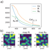 |
Fig. 1 (a) The three components set used to create a synthetic spectrum image − they have been extracted from an experimental dataset, (b)–(d) 64 × 64 maps obtained with the chequerboard model (8 × 8 blocks); each of these maps is associated with one component. |
 |
Fig. 2 The four components set used to create a synthetic spectrum image. They have been obtained by fitting spectra extracted from the dataset used in [2,30]. |
2.2 Unmixing algorithms
Before proceeding to unmixing, the number of endmembers has to be estimated, as this is a parameter used by the unmixing AE. Although various algorithms already exist for this estimation [35], the process remains a delicate task. The estimation is all the more difficult as the definition of endmembers is subjective and depends on the degree of precision to be attained. For example, if the Co in the sample had different degrees of oxidation, it is not clear if it would be necessary to distinguish metallic Co from Co2+ and Co3+. The number of endmembers also depends on the level of information sought and the experimental conditions of data acquisition (energy resolution for EELS spectroscopy). Estimating the number of endmembers is particularly difficult in remote sensing, where the sensor can uncover unknown target sources that cannot be identified a priori. However, this estimation process is different in microscopy, where the global composition of the sample, which is a manufactured material, is well known. On the other hand, including more endmembers will not immediately improve the quality of unmixing results. Thus, in reference [29], increasing the number of endmembers for the Urban image unmixing degrades the results for most tested AEs.
In this study, the number of endmembers for the synthetic images was the same as the number used to generate the data. As the sample composition was known for the experimental data, this physical information was part of the unmixing process. Thus each element present in the sample, i.e., Ru, Co and Pt, corresponded to one spectral signature and then to one endmember. This choice of the number of endmembers implied that any spectral variation occurring in the data was assimilated to noise.
The methods compared in this work are listed in Table 1.
Although many spectral unmixing algorithms exist, unmixing is not frequently used in the STEM-EELS domain. The algorithms most used are NMF and ICA − as implemented in the Toolbox Hyperspy − and VCA.
Hyperspy uses the Scikit-learn version of the NMF algorithm, sklearn.decomposition.NMF [36]. NMF decomposes the data matrix X by resolving the optimisation problem:

X being the data, L a loss function measuring the similarity between X and the decomposition, and W and H the matrices resulting from the decomposition. A regularisation term can be added to the loss function. Furthermore, the initialisation mode can be changed, as well as the distance. The default values provided in Hyperspy were kept (Frobenius norm, no regularisation, initialisation by Non-negative Double Singular Value Decomposition).
ICA decomposes X, assuming that the components are statistically independent [37,38]. Independency is a strong assumption whose relevance has been questioned in the remote sensing community [31,38]. It is a widely used method in STEM-EELS, probably due to its implementation from the first versions of Hyperspy. Hyperspy uses, by default, the Scikit-learn implementation, (https://scikit-learn.org/stable/modules/generated/sklearn.decomposition.FastICA.html#sklearn.decomposition.FastICA). This implementation is based on [39]. This default version was used in the present work.
VCA is one of the most advanced convex geometry-based endmember detection methods. It is based on successive projections on hyperplanes [31]. This algorithm assumes the presence of at least one pure pixel for each component in the data. If there is no pure pixel, it uses the highest quality pixel that is available. Although the pure pixel condition is not always verified in STEM-EELS HSIs, this algorithm is fast and computationally relatively light. VCA has been implemented in Python (https://github.com/Laadr/VCA) and Matlab (http://www.lx.it.pt/∼bioucas/code.htm). It is commonly used in the remote sensing community and is often used as a reference to evaluate new unmixing algorithms. It has already been used to unmix STEM-EELS SI [2,40,41].
BLU is a fully Bayesian algorithm which uses a Gibbs sampler algorithm to solve the unmixing problem without requiring the presence of pure pixels in SI [32]. Its performance for EELS HSIs has been evaluated in [2].
AEs can be used for unsupervised learning technique using neural networks to learn a latent space representation of the input. In this work, we used only AEs with small number of layers (typically less than four), and they belong to the domain of representation learning rather than traditional Deep Learning. The part of the network that compresses the input into the latent representation is called the encoder. The part that reconstructs the input from the latent representation is the decoder. The AE architecture imposes a bottleneck that forces a compressed input representation (Fig. 3).
The AE is trained by using the input as target data, meaning that the AE learns to reconstruct the original input. The decoder part of the AE aims to reconstruct the input from the latent space representation. By limiting the decoder to one layer, it has been shown that the activations of the last layer of the encoder correspond to the abundances and the weights of the decoder to the endmembers [23]. The encoder converts the input spectra to the corresponding abundance vectors, i.e., the output of the hidden layer. The decoder reconstructs the input from the compressed representation with the weights in the last linear layer interpreted as the endmember matrix [29]. The action of the last layer of the decoder can be written as:

where  is the output of the network (reconstructed spectrum), i.e., an estimation of the input xp, a(L-1) are the activations of the previous layer, W(L) are the weights of the output layer, L being the total number of layers, B the number of bands and R the number of endmembers.
a(L−1) is of dimension R×1 and W(L) is a B×R matrix, which has to be interpreted as abundances and endmembers for a given input. The weights are fixed once the network is trained, and the endmembers are determined for the whole dataset. The activations are dependent on the input (pixel) analyzed.
According to this principle, the decoder must be a single layer, and this simple structure might affect the performance of the AE; however, the experiments show that this AE performs well in unmixing the remote sensing data. Although several articles have proposed neural networks to achieve unmixing, the corresponding code is only sometimes published in parallel. This lack of information is detrimental, as not only is re-implementing the code time-consuming, but many implementation details, such as utility layers and hyperparameters values, are not specified in publications on the subject, while modifying these features can significantly alter the results. Recent efforts have started to mitigate this issue, and several codes are available on the web, e.g. uDAS on GitHub (https://github.com/aicip/uDAS). Although linked to the field of Deep learning by its keywords, uDAS is a shallow AE with only one encoding layer. Its architecture makes it somewhat close to a conventional optimisation method for an inverse problem, with an alternating optimisation of the encoder and the decoder [21].
DAEU [23] comprises an encoder with 4 Dense layers with Leaky ReLU activation functions, followed by utility layers (Batch Normalization, enforcing ASC SumToOne layer, Gaussian Dropout layer). The LMM constraints the architecture of the decoder which is a single layer. Objective function is spectral angle distance (SAD). This method performs better than the comparison methods (VCA, different NMF-based methods) for tested remote sensing data sets.
To take the spatial structure of the HSI into account, MTAEU [24] uses multiple parallel branches of unmixing autoencoders (AEs), each tasked with unmixing a whole patch. The inputs (patches) are concatenated and connected into a large shared hidden layer. The architecture branches again after this shared layer, and each autoencoder performs dimensional reduction. The activations for each autoencoder become the abundance fractions. However, all autoencoders use the same decoder to discover the same endmembers. The loss function is the SAD. MTAEU perform significantly better than DAEU and uDAS on remote sensing data sets.
The CNNAEU [25] employs 2-D convolutional layers with LeakyReLU activation, Batch Normalization, and Spatial Dropout. A Softmax function is applied to enforce the sum-to-one constraint on the abundances. The output of this layer can be interpreted as the abundance fractions. The final layer is a linear decoder layer that reconstructs the input patch. The loss function used is the SAD. CNNAEU is claimed to perform particularly well for endmembers extraction.
Implementations of DAEU (see Tab. 2), MTAEU and CNNAEU have been recently made available (https://github.com/burknipalsson/hu_autoencoders) with the corresponding publication [29].
The models for all the AEs evaluated in this work were those available online without changing the architecture or the hyperparameters.
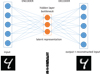 |
Fig. 3 Basic principle of an autoencoder. The hidden layer is a bottleneck that forces a compressed input representation. The input example is a 2D image from the MNIST dataset [42]. The 2D 28 × 28 pixels image is processed as a 784 vector. In our case, the input is a spectrum. |
Detail of layers of the encoder in DAEU network [23]. B is the number of channels of the input (spectrum). R is the number of units of the latent, hidden layer, i.e., the number of components to unmix. The utility layer performs an operation not specific to a neural network; in particular, the utility layer does not change the number of units.
3 Results and discussion
3.1 Unmixing of synthetic data
The results of the different unmixing algorithms are shown in Figures 4 and 5.
uDAS is the algorithm that gives the best results for both sets of synthetic data, three and four components. In contrast, ICA and NMF give the worst results. The others (VCA, BLU, DAEU, MTAEU, CNNAEU) produce intermediate-quality results. uDAS has the particularity of including denoising and regularisation constraints (ℓ2,1 on endmembers), which may explain the good results obtained. It should be noted that the chequerboard structure of synthetic images creates a non-zero proportion of pure pixels, which favours the use of VCA and uDAS (as it is initialised with VCA).
The results are qualitatively the same for ranking the algorithms in terms of performance for the two types of synthetic data: three components with 200 energy channels (Fig. 1) and four components with 903 energy channels (Fig. 2). Moreover, the spectra chosen to build the data are significantly different, with M and L edges (Fig. 1) versus K edges (Fig. 2), which does not influence the results significantly.
The SAD metric is scale-invariant and solely takes into account the shape of an extracted component. Its absolute amplitude can be very different from the reference endmember without affecting the result. In contrast, the NMSE metric will calculate a significant error for a calculated abundance map that does not respect the sum-to-one rule. NMF and ICA methods do not use this constraint, so they get a high error.
No significant improvement is observed in MTAEU and CNNAEU compared to DAEU, despite their higher complexity in accounting for the HSI spatial correlations between pixels. These methods utilize this spatial information by treating the input as a patch (a patch refers to a small block of pixels, typically a 3 × 3 square with 9 pixels).
Thus, while patch-based methods usually outperform conventional methods in image analysis, in this case spatial structure does not have an impact on the quality of unmixing for STEM-EELS HSIs.
The higher number of hyperparameters related to a complex architecture may require adjustment to the characteristics of the STEM-EELS HSIs, i.e., more energy channels and fewer pixels.
The computation times required by each algorithm are reported in Table 3 (3 GHz Intel® Core™i7-1185G7 − except for CNNAEU, which has been trained on a computer with a GPU NVIDIA Quadro RTX4000 8Go (7.5 Cuda score)). The complexity of VCA, ICA, and NMF is lower than those of DAEU, BLU and uDAS.
As the acquisition of the data is relatively fast, around 10 minutes for core loss data, even less with the new generation of direct detection detectors, the microscope user might want to process the data quickly, whether done after or online during the experiment on the microscope. During the acquisition time, using basic neural networks could allow the training to be carried out with a first data cube (or a previous one in the case of a series of experiments). Then one could apply the trained network to the following acquisitions, reducing the execution time to 0.1 seconds. The experimental conditions of STEM-EELS are thus particularly well adapted to using a neural network because these networks allow exploiting several HSIs acquired under the same conditions. This situation differs from the case of HSIs acquired in remote sensing, where the cases presented in the literature correspond to the exploitation of a single HSI. Even if the performance of AEs for spectral unmixing is currently limited, their use remains interesting in STEM-EELS because of their speed in inference.
 |
Fig. 4 Performance of different algorithms for abundances maps estimation with a log scale. ‘BS' is the background subtraction method. |
 |
Fig. 5 Performance of different algorithms for endmembers extraction (low score is better). |
Execution time (expressed in s) for different algorithms on synthetic data. For the AE, the time is the training time.
3.2 Experimental dataset
The different algorithms were applied to a HSI acquired on a Pt/Co/Ru/Pt multilayer [43]. These heterostructures were investigated regarding their magnetic properties, i.e., Dzyaloshinskii-Moriya interaction, at metallic interfaces. The nominal stacking corresponds to: Si/SiO2/Ta(10 nm)/Pt(8 nm)/Co(1.7 nm)/Ru(0.5 nm)/Pt(3 nm). In these samples, the Ru layer and its top and bottom interfaces, i.e., Pt/Ru and Ru/Co, respectively, can have an impact on the local magnetic properties of the stacking. Therefore, characterising this layer and the corresponding interfaces is essential. In particular, the Ru can diffuse into the Co layer, and it is thus necessary to establish a profile for Ru.
The data were acquired on a USTEM Nion microscope operated at 100 kV using a Medipix3 detector (Merlin EM Quantum Detector) with a 50 ms dwell time. The HSI is 60 × 75 pixels × 200 energy channels (Fig. 6). A pixel represents 0.12 × 0.12 nm and an energy channel 3.33 eV. Data were corrected for gain before any advanced processing.
As the Ru is a delayed M-edge (279 eV for M4,5), it was challenging to determine the maps using the BS and characteristic signal integration method used in EELS. Indeed, in EELS the typical method for obtaining an elemental map involves fitting the background with a power law over a specified energy interval and then subtracting this background. Finally, the signal is summed in a second energy window. This process is usually performed using a dedicated software such as Gatan DigitalMicrograph, as illustrated in Figure 7. In the case of Ru, we are unable to satisfactorily model the background under the Ru M4,5 edge (Fig. 7a), leading to non-physical negative intensity in some parts of the image (Fig. 7e). Therefore, using an unmixing method for this type of data was interesting. Nevertheless, the M2,3 edge of Ru was used to obtain intensity maps to compare with the maps obtained by unmixing. (Fig. 7d), as the M2,3 edge is detectable with the direct detection camera and the background can be successfully fit in this energy range (Fig. 7b).
The profiles in Figure 7 are obtained by summing three lines of pixels corresponding to 3.6 nm width at the top of the HSI. There is an artefact with a small non-zero intensity outside the Ru layer, depending on the pre-edge energy window selection.
The Pt-M edge is in a high-energy range (2122 eV), so this edge was not used in the unmixing process.
As it is a real sample, there is no available GT, so it was impossible to compute metrics for experimental data; then, the evaluation was qualitative. However, the profiles obtained by unmixing were compared with those obtained by the BS method. The following results are obtained with the processing of data of SI1, which is a restricted area of 60 × 75 pixels. The extracted components are presented in Figure 8.
The Co component is well-extracted in all cases. The components obtained by VCA, BLU and uDAS are very similar, probably because uDAS and BLU are initialised by VCA.
Ru component extraction is more challenging, and there is still a Co signal in all components except in the component extracted by DAEU. VCA relies on the pure pixel hypothesis, and there is probably no pure pixel corresponding to Ru. A remarkable result is that the DAEU neural network not only manages to remove the Co but obtains a component close to the reference edge obtained in [44]. Despite a very low dispersion (about 3.3 eV/channel), some fine structure is present on the Ru-M edge. Although they have much more complex architectures, MTAEU and CNNAEU do not manage to extract the Ru component more satisfactorily than DAEU in the case of SI1. The resulting maps are presented in Figure 9.
As we do not have ground truth for the experimental data, we relied on the maps obtained through continuous background subtraction and summation of the characteristic signal (BS) to assess the quality of the maps calculated by the unmixing methods. However, it did not seem feasible to use these BS maps for a quantitative evaluation, so our discussion of the results is based on a visual comparison. The maps obtained with NMF are visually the closest to those obtained by BS. The maps obtained by VCA, BLU and uDAS are satisfactory. DAEU, MTAEU and CNNAEU give very contrasting maps with a steep interface between the Co and Ru layers, which does not correspond to the physical reality. For DAEU and MTAEU, the abundances are close to either 0 or 1; this problem has been reported in the literature for this class of AEs [24]. Despite their complexity, MTAEU and CNNAEU do not perform better than DAEU on the experimental data. It might be necessary to adjust some hyperparameters, which is a complex task, as the networks are trained on the reconstruction quality rather than on the quality of the unmixing.
To obtain a more precise estimation of the quality of the unmixing, the profiles obtained by the different unmixing methods are presented in Figure 10. The profiles were obtained by summing three rows from the Ru maps, in the same way as the profiles presented in Figure 7. The Ru profile presents an asymmetry with diffusion in the Co layer.
If the unmixing is correctly performed, the shape of the profile should be close to those obtained by the BS method. The comparison of abundance profiles is a criterion that is not, to our knowledge, used in remote sensing, where one relies solely on metrics and the visual comparison of maps to evaluate the performance of different methods. As was the case for the maps, the profile obtained by NMF corresponds to the profile obtained by BS and appears close to physical reality. The profiles obtained by VCA and BLU are also satisfying. They are close to zero, far from the layer on the left part of the layer, while it was not possible to eliminate the signal by subtracting the background in front of the threshold. However, an anomaly is observed on the right side of the profile. Some degree of spectral variability (caused, for example, by variations in thickness) could explain why the algorithms have difficulty representing the data set with only three components.
uDAS somehow reproduces the asymmetry of the profile but shows a non-zero intensity away from the Ru layer. DAEU, MTAEU and CNNAEU fail to reproduce the asymmetry of the profile; thus, the weight of the Ru component falls to 0 in the region where it is mixed with Co. Therefore, the improved extraction of the Ru component by DAEU did not result in a satisfactory map.
The results obtained on the synthetic data are not fully applicable to the experimental data. Several limitations of synthetic SI can be identified. Firstly, these images are constructed very simply; spectral variability is not considered. Moreover, the synthetic chequerboard maps contain a certain proportion of pure pixels for each component. In contrast, in the experimental situation, one of the components (Ru) corresponds to almost no pure pixels. To elaborate synthetic data closer to reality would be necessary to obtain a relevant evaluation of the efficiency of the unmixing algorithms.
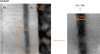 |
Fig. 6 HAADF image corresponding to the region where HSI acquisition was conducted. |
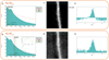 |
Fig. 7 Using the M4,5 edge (a) to map the Ru (c) produces negative values for intensities, as can be seen in the resulting profile (e). The M2,3 edge (b) gives better results (d). On the profile (f) there is an artefact with a small non-zero intensity outside the Ru layer. |
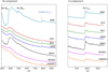 |
Fig. 8 Components obtained by the different unmixing algorithms tested on SI1. Each component corresponds to a unique edge, Ru-M and Co-L2,3. |
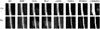 |
Fig. 9 Maps obtained by the different unmixing algorithms tested on SI1. As each component corresponds to a unique edge, they are elementary maps. |
 |
Fig. 10 Profiles through Ru maps presented in Figure 9. Intensities values (arbitrary units) have been re-scaled to match the ‘BS’ profile. |
4 Conclusions
This work demonstrates that AEs give interesting results for spectral unmixing. In particular, suitable extraction of the Ru component can be obtained despite the absence of pure pixels for this element in the experimental data. Moreover, the organisation of the STEM-EELS experiments makes them well adapted to Representation Learning: the network is trained on the first set of data (first acquired HSI) and then the weights are applied to the data acquired subsequently while benefiting from a swift execution time. This procedure can also apply if a series of very similar samples is studied (for example, in the case of Pt/Co/Ru sample by varying the thickness of the Ru layer).
More complex neural networks such as CNNAEU and MTAEU, which are efficient according to the literature in remote sensing [29], should be able to handle STEM-EELS data. However, they output worse results on our STEM-EELS data. One hypothesis is that this failure is due to the specific shape of the EELS spectra with a strong signal represented by the continuous background and relatively weak superimposed specific signals. Adapting either the hyperparameters (batch size, number of hidden units...) or the architecture would probably be necessary.
On the other hand, the results obtained on the experimental data are not as good as expected from the first tests on the synthetic data. The model used to create synthetic HSI is too simple, and introducing a degree of spectral variability would be helpful, for example by using a variational AE (VAE) [29] which encodes the input as a distribution.
Researchers continue to make progress on hyperspectral unmixing by Neural Networks. Such progress can be achieved through cooperative work in the field, in particular by allowing open access to the codes used [11].
Acknowledgments
We thank André Thiaville (LPS, Orsay), William Legrand, Nicolas Reyren and Vincent Cros (UMP CNRS/Thales, Palaiseau) for the Pt/Co/Ru data. We are grateful to Calvin Peck from Academic Writing Center (U. Paris Saclay) for his patience in editing the manuscript.
Funding
This project has been funded in part by the National Agency for Research under the program of future investment TEMPOS-CHROMATEM (reference no. ANR-10-EQPX-50) and by the European Union's Horizon 2020 research and innovation program under grant agreement No. 823717 (ESTEEM3).
Conflicts of interest
The authors have nothing to disclose.
Data availability statement
Data are available on request. The codes used are the ones cited in the references and are available on line.
Author contribution statement
Methodology, N. B., L. B. and G. L.; Data Acquisition, L. B.; Data Analysis, N. B., L. B. and G. L.; Writing − Original Draft Preparation, N. B.; Writing − Review & Editing, N.B., L. B..
References
- N. Bonnet, N. Brun, C. Colliex, Extracting information from sequences of spatially resolved EELS spectra using multivariate statistical analysis, Ultramicroscopy 77, 97 (1999), https://doi.org/10.1016/S0304-3991(99)00042-X [CrossRef] [Google Scholar]
- F. de la Peña, M.-H. Berger, J.-F. Hochepied, F. Dynys, O. Stephan, M. Walls, Mapping titanium and tin oxide phases using EELS: an application of independent component analysis, Ultramicroscopy 111, 169 (2011), https://doi.org/10.1016/j.ultramic.2010.10.001 [CrossRef] [PubMed] [Google Scholar]
- N. Dobigeon, N. Brun, Spectral mixture analysis of EELS spectrum-images, Ultramicroscopy 120, 25 (2012), https://doi.org/10.1016/j.ultramic.2012.05.006 [CrossRef] [PubMed] [Google Scholar]
- J.M. Bioucas-Dias, A. Plaza, N. Dobigeon et al., Hyperspectral unmixing overview: Geometrical, statistical, and sparse regression-based approaches, IEEE J. Sel. Top. Appl. Earth Observ. Remote Sens. 5, 354 (2012), https://doi.org/10.1109/JSTARS.2012.2194696 [CrossRef] [Google Scholar]
- S. Turner, R. Egoavil, M. Batuk et al., Site-specific mapping of transition metal-oxygen coordination in complex oxides, Appl. Phys. Lett. 101, 241910 (2012), https://doi.org/10.1063/1.4770512 [CrossRef] [Google Scholar]
- L. Ma, Y. Liu, X. Zhang, Y. Ye, G. Yin, B.A. Johnson, Deep learning in remote sensing applications: a meta-analysis and review, ISPRS J. Photogramm. Remote Sens. 152, 166 (2019), https://doi.org/10.1016/j.isprsjprs.2019.04.015 [CrossRef] [Google Scholar]
- L. Zhang, L. Zhang, B. Du, Deep learning for remote sensing data: a technical tutorial on the state of the art, IEEE Geosci. Remote Sens. Mag. 4, 22 (2016), https://doi.org/10.1109/MGRS.2016.2540798 [CrossRef] [Google Scholar]
- A. Signoroni, M. Savardi, A. Baronio, S. Benini, Deep learning meets hyperspectral image analysis: a multidisciplinary review, J. Imag. 5, 52 (2019), https://doi.org/10.3390/jimaging5050052 [CrossRef] [Google Scholar]
- X.X. Zhu, D. Tuia, L. Mou et al., Deep learning in remote sensing: a review, IEEE Geosci. Remote Sens. Mag. 5, 8 (2017), https://doi.org/10.1109/MGRS.2017.2762307 [CrossRef] [MathSciNet] [Google Scholar]
- O. Ronneberger, P. Fischer, T. Brox, U-Net: convolutional networks for biomedical image segmentation, in Medical Image Computing and Computer-Assisted Intervention − MICCAI 2015. MICCAI 2015. Lecture Notes in Computer Science, edited by N. Navab, J. Hornegger, W. Wells, A. Frangi (Springer, Cham, 2015), vol 9351. https://doi.org/10.1007/978-3-319-24574-4_28 [Google Scholar]
- N. Audebert, B. Le Saux, S. Lefèvre, Deep learning for classification of hyperspectral data: a comparative review, IEEE Geosci. Remote Sens. Mag. 7, 159 (2019), https://doi.org/10.1109/MGRS.2019.2912563 [CrossRef] [Google Scholar]
- M. Wang, M. Zhao, J. Chen, S. Rahardja, Nonlinear unmixing of hyperspectral data via deep autoencoder networks, IEEE Geosci. Remote Sens. Lett. 16, 1467 (2019), https://doi.org/10.1109/LGRS.2019.2900733 [CrossRef] [Google Scholar]
- M. Zhao, M. Wang, J. Chen, S. Rahardja, Hyperspectral Unmixing via Deep Autoencoder Networks for a Generalized Linear-Mixture/Nonlinear-Fluctuation Model, arXiv:1904.13017, https://doi.org/10.48550/arXiv.1904.13017 [Google Scholar]
- M. Zhao, M. Wang, J. Chen, S. Rahardja, Hyperspectral unmixing for additive nonlinear models with a 3-D-CNN autoencoder network, IEEE Trans. Geosci. Remote Sens. 60, 1 (2021), https://doi.org/10.1109/TGRS.2021.3098745 [CrossRef] [Google Scholar]
- S. Shi, M. Zhao, L. Zhang, J. Chen, Variational autoencoders for hyperspectral unmixing with endmember variability, in ICASS P 2021–2021 IEEE International Conference on Acoustics, Speech and Signal Processing (ICASSP) (Toronto, ON, Canada, 2021), p. 1875, https://doi.org/10.1109/ICASSP39728.2021.9414940. [Google Scholar]
- H. Li, R.A. Borsoi, T. Imbiriba, P. Closas, J.C. Bermudez, D. Erdoğmuş, Model-based deep autoencoder networks for nonlinear hyperspectral unmixing, IEEE Geosci. Remote Sens. Lett. 19, 1 (2021), https://doi.org/10.1109/LGRS.2021.3075138 [Google Scholar]
- S. Ozkan, B. Kaya, G.B. Akar, Endnet: Sparse autoencoder network for endmember extraction and hyperspectral unmixing, IEEE Trans. Geosci. Remote Sens. 57, 482 (2018), https://doi.org/10.1109/TGRS.2018.2856929 [Google Scholar]
- Y. Su, A. Marinoni, J. Li, J. Plaza, P. Gamba, Stacked nonnegative sparse autoencoders for robust hyperspectral unmixing, IEEE Geosci. Remote Sens. Lett. 15, 1427 (2018), https://doi.org/10.1109/LGRS.2018.2841400 [CrossRef] [Google Scholar]
- Y. Su, J. Li, A. Plaza, A. Marinoni, P. Gamba, S. Chakravortty, DAEN: deep autoencoder networks for hyperspectral unmixing, IEEE Trans. Geosci. Remote Sens. 57, 4309 (2019), https://doi.org/10.1109/TGRS.2018. 2890633 [CrossRef] [Google Scholar]
- S. Zhang, Y. Su, X. Xu, J. Li, C. Deng, A. Plaza, Recent advances in hyperspectral unmixing using sparse techniques and deep learning, in Hyperspectral Image Analysis, edited by S. Prasad, J. Chanussot (Springer, 2020), p. 377, https://doi.org/10.1007/978-3-030-38617-7_13 [Google Scholar]
- Y. Qu, H. Qi, uDAS: An untied denoising autoencoder with sparsity for spectral unmixing, IEEE Trans. Geosci. Remote Sens. 57, 1698 (2018), https://doi.org/10.1109/TGRS.2018.2868690 [Google Scholar]
- F. Palsson, J. Sigurdsson, J.R. Sveinsson, M.O. Ulfarsson, Neural network hyperspectral unmixing with spectral information divergence objective, in 2017 IEEE International Geoscience and Remote Sensing Symposium (IGARSS) (Fort Worth, TX, USA, 2017), p. 755, https://doi.org/10.1109/IGARSS.2017.8127062. [Google Scholar]
- B. Palsson, J. Sigurdsson, J.R. Sveinsson, M. O. Ulfarsson, Hyperspectral unmixing using a neural network autoencoder, IEEE Access 6, 25646 (2018), https://doi.org/10.1109/ACCESS.2018.2818280 [CrossRef] [Google Scholar]
- B. Palsson, J.R. Sveinsson, M.O. Ulfarsson, Spectral-spatial hyperspectral unmixing using multitask learning, IEEE Access 7, 148861 (2019), https://doi.org/10.1109/ACCESS.2019.2944072 [CrossRef] [Google Scholar]
- B. Palsson, M.O. Ulfarsson, J. R. Sveinsson, Convolutional autoencoder for spectral-spatial hyperspectral unmixing, IEEE Trans. Geosci. Remote Sens. 59, 535 (2021), https://doi.org/10.1109/TGRS.2020.2992743 [CrossRef] [Google Scholar]
- M. Zhao, S. Shi, J. Chen, N. Dobigeon, A 3-d-cnnframework for hyperspectral unmixing with spectral variability, IEEE Trans. Geosci. Remote Sens. 60, 1 (2022), https://doi.org/10.1109/TGRS.2022.3141387 [CrossRef] [Google Scholar]
- S. Shi, L. Zhang, Y. Altmann, J. Chen, Deep generative model for spatial-spectral unmixing with multiple endmember priors, IEEE Trans. Geosci. Remote Sens. 60, 1 (2022), https://doi.org/10.1109/TGRS.2022.3168712 [CrossRef] [Google Scholar]
- P. Ghosh, S.K. Roy, B. Koirala, B. Rasti, P. Scheunders, Hyperspectral unmixing using transformer network, IEEE Trans. Geosci. Remote Sens. 60, 1 (2022), https://doi.org/10.1109/TGRS.2022.3196057 [CrossRef] [Google Scholar]
- B. Palsson, J.R. Sveinsson, M.O. Ulfarsson, Blind hyperspectral unmixing using autoencoders: a critical comparison, IEEE J. Sel. Top. Appl. Earth Obs. Remote Sens. 15, 1340 (2022), https://doi.org/10.1109/JSTARS.2021. 3140154 [CrossRef] [Google Scholar]
- HyperSpy: Multi-dimensional data analysis toolbox — HyperSpy, https://doi.org/10.5281/zenodo.592838. Available: https://hyperspy.org/index.html (visited on 09/28/2022) [Google Scholar]
- J.M.P. Nascimento, J.M.B. Dias, Vertex component analysis: a fast algorithm to unmix hyperspectral data, IEEE Trans. Geosci. Remote Sens. 43, 898 (2005), https://doi.org/10.1109/TGRS.2005.844293 [CrossRef] [Google Scholar]
- N. Dobigeon, S. Moussaoui, M. Coulon, J.-Y. Tourneret, A.O. Hero, Joint Bayesian endmember extraction and linear unmixing for hyperspectral imagery, IEEE Trans. Signal Process. 57, 4355 (2009), https://doi.org/10.1109/TSP.2009.2025797 [CrossRef] [MathSciNet] [Google Scholar]
- L. Miao, H. Qi, Endmember extraction from highly mixed data using minimum volume constrained nonnegative matrix factorization, IEEE Trans. Geosci. Remote Sens. 45, 765 (2007), https://doi.org/10.1109/TGRS.2006.888466 [CrossRef] [Google Scholar]
- R. Arenal, F. de la Peña, O. Stéphan et al., Extending the analysis of EELS spectrum-imaging data, from elemental to bond mapping in complex nanostructures, Ultramicroscopy 109, 32 (2008), https://doi.org/10.1016/j.ultramic.2008.07.005 [CrossRef] [PubMed] [Google Scholar]
- C.I. Chang, Q. Du, Estimation of number of spectrally distinct signal sources in hyperspectral imagery, IEEE Trans. Geosci. Remote Sens. 42, 608 (2004), https://doi.org/10.1109/TGRS.2003.819189 [CrossRef] [Google Scholar]
- F. Pedregosa, G. Varoquaux, A. Gramfort et al., Scikit-learn: machine learning in Python, J. Mach. Learn. Res. 12, 2825 (2011) [MathSciNet] [Google Scholar]
- N. Bonnet, D. Nuzillard, Independent component analysis: a new possibility for analysing series of electron energy loss spectra, Ultramicroscopy 102, 327 (2005), https://doi.org/10.1016/j.ultramic.2004.11.003 [CrossRef] [PubMed] [Google Scholar]
- J.M.P. Nascimento, J.M.B. Dias, Independent component analysis applied to unmixing hyperspectral data, Proc. SPIE 5238, 306 (2004), https://doi.org/10.1117/12.510652 [CrossRef] [Google Scholar]
- A. Hyvärinen, E. Oja, Independent component analysis: algorithms and applications, Neural Netw. 13, 411 (2000), https://doi.org/10.1016/S0893-6080(00)00026-5 [CrossRef] [Google Scholar]
- I. Palacio, A. Celis, M.N. Nair et al., Atomic structure of epitaxial graphene sidewall nanoribbons: flat graphene, miniribbons, and the confinement gap, Nano Lett. 15, 182 (2015), https://doi.org/10.1021/nl503352v [CrossRef] [PubMed] [Google Scholar]
- M. Duchamp, M. Lachmann, C. Boothroyd et al., Compositional study of defects in microcrystalline silicon solar cells using spectral decomposition in the scanning transmission electron microscope, Appl. Phys. Lett. 102, 133902 (2013), https://doi.org/10.1063/1.4800569 [CrossRef] [Google Scholar]
- Y. LeCun, L. Bottou, Y. Bengio, P. Haffner, Gradient-based learning applied to document recognition, Proc. IEEE 86, 2278 (1998), https://doi.org/10.1109/5.726791 [CrossRef] [Google Scholar]
- W. Legrand, Y. Sassi, F. Ajejas et al., Spatial extent of the dzyaloshinskii-moriya interaction at metallic interfaces, Phys. Rev. Mater. 6, 024408 (2022), https://doi.org/10.1103/PhysRevMaterials.6.024408 [CrossRef] [Google Scholar]
- D. Muller, Ruthenium Bulk M2,3 and M4,5, Appl. Phys. Group @ Cornell. [Online] Available: https://muller.research.engineering.cornell.edu/spectra/ruthenium-bulk-m23-and-m45/ (visited on 02/24/2023) [Google Scholar]
Cite this article as: Nathalie Brun, Guillaume Lambert, Laura Bocher, EELS hyperspectral images unmixing using autoencoders, Eur. Phys. J. Appl. Phys. 99, 28 (2024)
All Tables
Detail of layers of the encoder in DAEU network [23]. B is the number of channels of the input (spectrum). R is the number of units of the latent, hidden layer, i.e., the number of components to unmix. The utility layer performs an operation not specific to a neural network; in particular, the utility layer does not change the number of units.
Execution time (expressed in s) for different algorithms on synthetic data. For the AE, the time is the training time.
All Figures
|
Fig. 1 (a) The three components set used to create a synthetic spectrum image − they have been extracted from an experimental dataset, (b)–(d) 64 × 64 maps obtained with the chequerboard model (8 × 8 blocks); each of these maps is associated with one component. |
| In the text | |
|
Fig. 2 The four components set used to create a synthetic spectrum image. They have been obtained by fitting spectra extracted from the dataset used in [2,30]. |
| In the text | |
|
Fig. 3 Basic principle of an autoencoder. The hidden layer is a bottleneck that forces a compressed input representation. The input example is a 2D image from the MNIST dataset [42]. The 2D 28 × 28 pixels image is processed as a 784 vector. In our case, the input is a spectrum. |
| In the text | |
|
Fig. 4 Performance of different algorithms for abundances maps estimation with a log scale. ‘BS' is the background subtraction method. |
| In the text | |
|
Fig. 5 Performance of different algorithms for endmembers extraction (low score is better). |
| In the text | |
|
Fig. 6 HAADF image corresponding to the region where HSI acquisition was conducted. |
| In the text | |
|
Fig. 7 Using the M4,5 edge (a) to map the Ru (c) produces negative values for intensities, as can be seen in the resulting profile (e). The M2,3 edge (b) gives better results (d). On the profile (f) there is an artefact with a small non-zero intensity outside the Ru layer. |
| In the text | |
|
Fig. 8 Components obtained by the different unmixing algorithms tested on SI1. Each component corresponds to a unique edge, Ru-M and Co-L2,3. |
| In the text | |
|
Fig. 9 Maps obtained by the different unmixing algorithms tested on SI1. As each component corresponds to a unique edge, they are elementary maps. |
| In the text | |
|
Fig. 10 Profiles through Ru maps presented in Figure 9. Intensities values (arbitrary units) have been re-scaled to match the ‘BS’ profile. |
| In the text | |
Current usage metrics show cumulative count of Article Views (full-text article views including HTML views, PDF and ePub downloads, according to the available data) and Abstracts Views on Vision4Press platform.
Data correspond to usage on the plateform after 2015. The current usage metrics is available 48-96 hours after online publication and is updated daily on week days.
Initial download of the metrics may take a while.