| Issue |
Eur. Phys. J. Appl. Phys.
Volume 85, Number 3, March 2019
|
|
|---|---|---|
| Article Number | 30701 | |
| Number of page(s) | 8 | |
| Section | Imaging, Microscopy and Spectroscopy | |
| DOI | https://doi.org/10.1051/epjap/2019180297 | |
| Published online | 26 April 2019 | |
https://doi.org/10.1051/epjap/2019180297
Regular Article
Speckle decorrelation with wavelength shift as a simple way to image transport mean free path
1
Univ Rennes, CNRS, Institut de Physique de Rennes, UMR 6251, Rennes, France
2
Univ Rennes, CNRS, Institut FOTON, UMR 6082, Rennes, France
* e-mail: This email address is being protected from spambots. You need JavaScript enabled to view it.
Received:
5
October
2018
Received in final form:
8
January
2019
Accepted:
4
February
2019
Published online: 26 April 2019
Abstract
We present an experimental scheme for determining the light transport properties of random disordered materials. The sample is illuminated with a laser and the speckle patterns obtained at different wavelengths are recorded with a camera. The transport mean free path is then deduced from the correlation functions of the scattered intensities. This method is tested on two kinds of random materials: colloidal particles dispersed into a polymeric matrix and on granular material made of glass beads. The possibility to image a material with a disorder varying at large scale is finally presented.
© A. Mikhailovskaya et al. published by EDP Sciences, 2019
 This is an Open Access article distributed under the terms of the Creative Commons Attribution License (http://creativecommons.org/licenses/by/4.0), which permits unrestricted use, distribution, and reproduction in any medium, provided the original work is properly cited.
1 Introduction
The transport of radiation into a multiply scattering medium may be accurately described within the diffusion approximation [1–3]. The knowledge of the corresponding diffusion coefficient into the sample is important for at least two major reasons. First, its value is linked with the internal structure of the scattering medium [4–6], which opens interesting applications in soft matter studies and in the biomedical domain for imaging through scattering tissues [7–12]. Secondly, the light diffusion coefficient drives the probability for photons to follow a given path into the sample. It is a fundamental parameter for spectroscopic methods, such as the Diffusing Wave Spectroscopy (DWS) [13,14], which assesses the dynamical processes in scattering samples.
Different techniques have been used to measure the diffusion coefficient of light (or the related transport mean free path (TMFP) l *) into a scattering medium, which may be classified in the following way [15]:
If the medium has a known temporal dynamics, the characteristic timescale of the fluctuations of the scattered intensity depends on the probability of path lengths, which in turns depends on l *.
-
(ii)
Response to a known illumination pattern [4]
The medium is illuminated locally, and the spatial profile of the backscattered intensity is measured [4,5]. l * may be determined from the comparison with theoretical predictions [19]. Illumination with random patterns is also possible [20,21]
-
(iii)
Coherent backscattering cone [22]
At very small angles around the backscattering direction, the scattered intensity is increased due to interferences between different reverse paths. This intensity enhancement occurs into a cone whose width depends on l *.
The transmission of the light through a slab of the scattering medium is measured as a function of its thickness. l * may be obtained by fitting the transmission with the appropriate theoretical expression.
A light pulse entering into a diffusive material is broadened during its propagation due to the distribution of path lengths. Practical use of this method is hindered when the typical broadening time is smaller than the nanosecond, and a mode-locked laser is needed.
As a complementary approach to the above technique, an intensity-modulated light (∼100 MHz to ∼100 GHz) can be used. Depending on the scattering properties of the medium and its thickness, the detected modulated light has a reduced modulation index and an additional phase, allowing the scattering parameters to be estimated [7,28].
This last technique relies on the measurement of intensity correlations between speckle patterns obtained at different frequencies of illumination, from which the l * value can be retrieved. We will use this method in our study, and we will describe it extensively in the following.
Although numerous papers report the measurement of l *, there is, to our knowledge, no systematic comparisons between those different methods in the literature. The reason is that the precision of the extracted l * values significantly differs depending of the method. DWS method (i) is widely used, but needs a system with a known internal dynamics, excluding any static systems. The method (ii) that exploits the properties of the diffusion equation in backscattering geometry is sensitive to the boundary conditions [4], whereas transmission geometries which probe the bulk of the sample are less dependent on boundary conditions. The shape of the enhanced backscattering cone, used in (iii), is difficult to obtain due to many experimental drawbacks [22]. The commonly used method of static transmission (iv) needs a sample of a given thickness, which may imply the destruction by cutting the sample into slices and doesn't allow remote and quick measurements. Moreover, the variation of the scattered intensity with the angular direction is dependent on the scattering material [31]. So the transmitted intensity can only be obtained by integration of the scattered intensity on a full half-space (2π sr). The use of (v) needs pulsed laser, a setup which is not easily accessible. The methods (vi) and (vii) may be viewed as analogous to DWS techniques. In DWS, the phase shifts are due to the internal dynamics of the sample, and temporal correlation functions are measured. In (vi) and (vii), the phase shifts are due to an external change of the frequency or wavelength. Methods (vi) and (vii) may also be used in any scattering geometries, including transmission and backscattering. An important advantage of the backscattering geometry [32] is that it enables to transpose to imaging scenarios, where one aims at resolving the spatial distribution of the diffusion coefficient or the TMFP. It should be noted that when a diffusing material is illuminated, the light penetrates inside the material, and this holds even in a backscattering geometry. This situation is different from scattering from a rough surface where the changes of the path length with a variation of wavelength are due to the roughness of the surfaces [33,34].
The time of flight and wavelength correlations measurements are not frequently used, mostly due to the expensive cost of tunable laser sources. We demonstrated in a previous study that cheap tunable He–Ne gas lasers may be used in this method [30]. In this experiment, the laser frequency was tuned by changing the cavity length of a single longitudinal mode laser. The drawback of this laser source was the very small range of laser frequency shift. In the present study, we report the use of an easily available near infrared laser diode at telecom wavelength (1.55 μm). The cavity length, and hence the laser frequency shift may be largely tuned without mode hopping. As we shall demonstrate in this article, the use of such laser source allows to perform l * measurements very easily, and also enables imaging of the TMFP of scattering materials.
The paper is organized in the following way. We first begin with a theoretical part which recalls the principle of wavelength shift measurements. Analytical expressions for correlation functions in the backscattering geometry are given. In the next section, we present the experimental setup used and a typical raw experimental measurement. We then perform experiments on two different kinds of scattering materials: TiO2 particles dispersed into PDMS gel and packing of dielectric spheres, and we analyze the data into the theoretical framework. Finally, we present in the last section a modification of the setup showing that the spatial variations of the transport mean free path may be imaged with this technique.
2 Theory
2.1 Principle of the experiment
We consider the propagation of light into a heterogeneous medium. Due to the scattering, the light follows various optical paths while propagating in the material as shown schematically in Figure 1a. At a given observation point, the electromagnetic field can be expressed as a sum on the different paths:  , where j labels a given path, E
j
the amplitude of the scattered electromagnetic field along the path j ,
, where j labels a given path, E
j
the amplitude of the scattered electromagnetic field along the path j ,  is the phase shift between the observation and the illumination points, and λ the optical wavelength. We now vary the optical wavelength, and let
  denote the new electromagnetic field. The product of the two fields is:
 (1a)
(1a)
 (1b)
(1b)
 (1c)
(1c)
When averaged on many different observation points, we obtain: (2)
with
(2)
with  . We suppose for this that the phase differences
  are uniformly distributed on [0 ;2π]. This assumption holds for the light emerging from a highly diffusing material because the path lengths of photons are very large compared to λ in this case.
The normalized correlation function  is then:
 (3)
(3)
The phase shift may be expressed as  , where s
j
is the path length and
, where s
j
is the path length and  the refractive index of the material. It follows that
  , and we note wavelength modulation
  . Taking the normalized distribution of optical path length P (s), we finally obtain, by replacing the discrete summation on the various paths by an integral:
 (4)
(4)
The correlation function of the scattered electromagnetic field can be obtained from the distribution of the photon path length using the Fourier transformation.
 |
Fig. 1 (a) Schematic view of the light propagation inside a highly diffusing material. (b) Boundary condition for the density of photons inside the material. The beam behaves as a point source located at a distance z 0 inside the material, and the density of photons extrapolates to 0 at a distance ze outside the material. |
2.2 Propagation into a scattering medium
When light propagates through a highly scattering material, the photons follow different optical paths that consist in multiple scattering events. Their trajectories can be represented as a random walk and therefore the light propagation can be described as a diffusion of photons in the material. The path length distribution P(s) is then linked to the diffusion coefficient (or the related transport mean free path l *) of the light. Theoretical analysis shows that the bulk propagation of light into the medium depends on the TMFP and on the absorption properties of the material given by the absorption length la . The boundary conditions of the diffusion equation set two other length-scales shown in Figure 1b. The first one is the location of the source of the diffusing intensity at the distance z
0 inside the illuminated face, which is commonly assumed to be equal to  [18]. The second one is the extrapolation length z
e
that sets the diffuse photon concentration field. z
e
depends on the refractive nature of the sample boundary [31] and is of the order of a few l
*. In the present experimental conditions, we used z
e
= 1.9l * (see below). Solving the diffusion equation for the light propagation with the right boundary conditions enables to determine P (s). This function depends on the experimental geometry such as transmission though a parallel slab or backscattering. For the particular case of backscattering from a semi-infinite half-space without absorption
[18]. The second one is the extrapolation length z
e
that sets the diffuse photon concentration field. z
e
depends on the refractive nature of the sample boundary [31] and is of the order of a few l
*. In the present experimental conditions, we used z
e
= 1.9l * (see below). Solving the diffusion equation for the light propagation with the right boundary conditions enables to determine P (s). This function depends on the experimental geometry such as transmission though a parallel slab or backscattering. For the particular case of backscattering from a semi-infinite half-space without absorption  , the Laplace transform of the path length distribution f (p) = ∫ P (s) e
ps
ds may be expressed as [17,35]:
, the Laplace transform of the path length distribution f (p) = ∫ P (s) e
ps
ds may be expressed as [17,35]: (5)and the correlation function (4) is therefore:
 (6)
(6)
Because the mean phase shift  is not zero, this correlation function is complex. However, in practice one does not measure the amplitude of the electric field but the intensity of the scattered light. The normalized correlation function of the scattered intensity is defined as:
 (7)
(7)
If the phase Φ
j
is uniformly distributed on [0 ;2π], then g
I
= 1 + β|g
E
|2, with β a numerical factor depending on the polarisation of the scattered fields  . We then finally obtain:
 (8)
(8)
In the case where some light absorption takes place, the correlation function may be calculated [30,36], with the following limit behaviors: (9a)
(9a)
 (9b)
(9b)
3 Experimental section
3.1 Optical setup
The experimental setup used is sketched in Figure
2. It represents a conventional arrangement of DWS in backscattering configuration. As an illumination source, we used a fibred distributed feedback (DFB) laser (1) commonly used for fibred telecommunications applications at 1.55 μm. Combined with a quality laser control unit, it was possible to modulate the incident wavelength from 1555.70 nm to 1557.05 nm without mode hopping by finely tuning the temperature of the semiconductor laser chip. We used a “butterfly” laser module (PowerSource 1905 LMI), containing the DFB laser (Avanex, USA) with the laser diode controller (LDC-3744, ILX LightWave, USA) to tune the wavelength and the power of the emitted light. With such a source, we may vary  over 8.5 × 10⁻⁴ with steps of 1.1 × 10⁻⁵. The spectral width of the laser diode is <5 MHz, giving a coherence length >60 m which is very large compared to the total path length inside the material. This means that the contrast of the speckle pattern does not dependent on the spectral width of the laser. Using an illumination in the near infrared diapason requires a special type of detector (4). We recorded the intensity fluctuations (speckle pattern) with an InGaAs short-wave infrared (SWIR) camera (OWL 320, Raptor Photonics, Northern Ireland) that provides 318 px × 254 px resolution with a pixel size of 15 μm × 15 μm. Together with the sample slab (3), this set of components is enough to retrieve the value of l * without spatial resolution. The quantity |g
E
|2 is obtained from the scattered intensities I
1 and I
2 at wavelength λ and λ + Δλ:
over 8.5 × 10⁻⁴ with steps of 1.1 × 10⁻⁵. The spectral width of the laser diode is <5 MHz, giving a coherence length >60 m which is very large compared to the total path length inside the material. This means that the contrast of the speckle pattern does not dependent on the spectral width of the laser. Using an illumination in the near infrared diapason requires a special type of detector (4). We recorded the intensity fluctuations (speckle pattern) with an InGaAs short-wave infrared (SWIR) camera (OWL 320, Raptor Photonics, Northern Ireland) that provides 318 px × 254 px resolution with a pixel size of 15 μm × 15 μm. Together with the sample slab (3), this set of components is enough to retrieve the value of l * without spatial resolution. The quantity |g
E
|2 is obtained from the scattered intensities I
1 and I
2 at wavelength λ and λ + Δλ: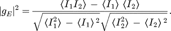 (10)
(10)
We take for this g I = 1 + β|g E |2 and g E (ε = 0) = 1, so that β = 〈I 2〉/〈 I 〉 2 − 1. In practice, we found a coherence factor β ≃ 0.41 which is slightly below the theoretical value β = 0.5 expected for an unpolarized scattered light. We made sure that this value varies only of few percent if the speckle size is larger than 2 pixels. This latter experimental condition was kept throughout the experiments reported below.
For the experiment in the imaging regime, the laser beam was expanded with a diverging lens (2) to illuminate fully the probing sample area. The image of the sample surface was formed using a lens (5) with a magnification ratio γ t = 0.2 on the camera sensor, and the average size of a speckle spot was set to approximately 3 pixels per speckle by adjusting the aperture of a diaphragm (6) in front of the camera. The spatial resolution was obtained by dividing the registered images in square zones of N × N pixels of the camera matrix. The correlation function was then calculated for these metapixels using equation (10). In the last section of this article, we also provide the analysis of a reasonable size of metapixels balancing the resolution quality of the estimated TMFP image and the measurement precision.
 |
Fig. 2 Experimental set-up: (1) DFB laser, (2) expanding lens, (3) sample slab, (4) infrared camera, (5) objective lens, (6) diaphragm. |
3.2 Scattering material preparation and properties
Two different kinds of scattering samples have been investigated.
The first kind consists of colloidal particles fixed in PDMS matrix. The procedure of their preparation was taken from [37]. The scattering particles are TiO2 (mon-droguiste.com, mean diameter d = 0.3 μm) and the PDMS kit is Sylgard 184 Silicone Elastomer from Dow Corning Corporation, Germany. Following [37], the particles were dispersed into the curing agent which was then mixed with the elastomer. The volume fraction of the particles into PDMS has been chosen as 3.4 × 10⁻⁴ and 1.3 × 10⁻³ so that the expected difference in the value of l * is approximately 4 times for the two samples prepared. The higher the particle content, the more opaque is the material. Therefore, to differentiate the samples in the following, we will refer to the one with lower volume fraction of TiO2 as turbid slab, and to the one with the higher volume fraction as white slab. The samples have been prepared in such a mold that the sample face has the dimensions of 6.5 cm × 6.5 cm and the final thickness of the samples is 9 mm and 19 mm for the white and for the turbid samples, respectively. Since the size polydispersity of the TiO2 particles is not well known, we could not compute l * from Mie theory. We then measured l * with an absolute transmission method detailed in Appendix A. The measured values of the transport mean free path with this reference experiment were  for the turbid sample, and
  for the white sample. The PDMS refraction index at the operating wavelength is n = 1.39 [38]. We supposed that the absorption is only due to the PDMS matrix. Indeed the TiO2 absorption is negligible, and in contrast to [37], we did not add any ink into the PDMS during preparation of the sample. Spectroscopic data gives a tabulated absorption length for PDMS of l
a
= 27.7 mm [38].
for the white sample. The PDMS refraction index at the operating wavelength is n = 1.39 [38]. We supposed that the absorption is only due to the PDMS matrix. Indeed the TiO2 absorption is negligible, and in contrast to [37], we did not add any ink into the PDMS during preparation of the sample. Spectroscopic data gives a tabulated absorption length for PDMS of l
a
= 27.7 mm [38].
The second kind of investigated samples is a dense packing of dielectric spheres. The beads (obtained from Silibeads) are made of sodalime glass and are dispersed in air. Two sizes of beads with mean diameter of  and
and  have been used. Together with other amorphous media such as foams, emulsions and porous materials, they form a broad class of scattering materials that can be represented as a packing of particles that are large compared to the optical wavelength. When propagated through such materials, photons also perform a random walk reaching the diffusive limit. In this case, the light transport is described by the geometrical optics, if
  , where
  is the difference of refractive indices between the beads
  and the surrounding medium
  . The model links the two lengthscales,
  and d, through a non-dimensional function
  of both refractive indices and of the solid volume fraction of the particles φ. In the case of a 3D packing of solid spheres this function has been obtained numerically using a ray-tracing algorithm [39]. For glass beads (
 ) in air (
 ) at φ = 0.64, it is found
  . Absorption lengths are unknown.
4 Experimental results
4.1 Measurements of homogeneous samples
We first discuss the experiments performed on the samples containing particles of TiO2 embedded in the PDMS matrix. In this case the particles are fixed, there is no Brownian motion and the scattered speckle pattern is static. However, the modulation of the incident wavelength introduces a variation in the optical path lengths, and hence a variation of the scattered intensity. As a consequence, the corresponding decorrelation of the signal can be followed using function g
I
of equation (7). The loss of correlation with the imposed shift in ε is shown in Figure
3 with symbols. The data is presented in the coordinates  , which naturally emerge from equation (8). For small values of
  (typically
  ),
),  , which corresponds to the small ε limit (see Eq. (9a)). For larger values of ε,
  decays linearly with
  in agreement with equation (9b). The slope of the decay is different for the “turbid” and the “white slab”, highlighting directly the difference in l *.
We have fitted the experimental data presented in Figure 3 with the theoretical expression of equation (8). The corresponding curves are shown with lines of the same graph. We have taken the refractive index of the scattering medium to be equal to the value  = 1.39 for the PDMS bulk, since the volume fraction of the colloidal particles is too low to affect it. The value of z
e
depends on the sample boundary reflectivity and, under given conditions, is approximately equal to 1.9
= 1.39 for the PDMS bulk, since the volume fraction of the colloidal particles is too low to affect it. The value of z
e
depends on the sample boundary reflectivity and, under given conditions, is approximately equal to 1.9  [31].
[31].
The retrieved values of TMFP are  for the “white” sample, and
  for the “turbid” sample. The uncertainty is obtained by varying the fitting range and measuring the difference between extracted values of fitting parameters. Those values may be compared with those obtained with the static transmission method, i.e.
  for the “white” sample, and
 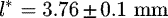 for the “turbid” sample. The absorption length l
a
has been taken as another adjusting parameter for the fitting procedure. We expect that the light is mostly absorbed by PDMS and therefore, the value of l
a
should be close for both samples. This is also visible from Figure
3: the shift that originates from the absorption and precedes the linear decay is quite similar for both curves. Indeed, the retrieved values are in agreement: 17.4 ± 0.9 mm for the “white” slab and 15.9 ± 0.9 mm for the “turbid” one.
for the “turbid” sample. The absorption length l
a
has been taken as another adjusting parameter for the fitting procedure. We expect that the light is mostly absorbed by PDMS and therefore, the value of l
a
should be close for both samples. This is also visible from Figure
3: the shift that originates from the absorption and precedes the linear decay is quite similar for both curves. Indeed, the retrieved values are in agreement: 17.4 ± 0.9 mm for the “white” slab and 15.9 ± 0.9 mm for the “turbid” one.
The obtained results demonstrate that the proposed technique allows the TMFP  to be easily and directly measured by modulating the wavelength of the illumination source. The method is rapid, not destructive and doesn't require any special sample preparation, and therefore, it can be applied to a broad range of materials.
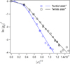 |
Fig. 3 Decorrelation of the scattered intensity with the wavelength modulation of the incident light for the samples of TiO2 particles embedded in PDMS matrix. Symbols stand for the experimental points and the lines correspond to the fitting curves obtained from equation (8): blue circles − “turbid slab”, black squares − “white slab”. |
4.2 Spatially resolved measurements
As an interesting extension of this method, we investigate its ability to measure the spatial variations of l * in a backscattering geometry. In this section we perform imaging measurements on granular materials that are disordered samples. The material is illuminated as described at the end of Section 3.1, and the backscattered light is still recorded by the camera. The correlation function g
I
is then calculated for each square zone (so called metapixel) of N × N pixels following equation (7). We first consider experiments performed on a “homogeneous sample” with only one value of the TMFP. This sample is composed of one kind of glass beads with a mean diameter  .
.
Figure
4a shows the correlation function for 6 different metapixels, the size of the metapixel beeing set to N × N = 96 × 96 pixels. We may notice that all correlation functions decrease with ε, but they decay to different and non-vanishing values for large ε. This may be linked with the light detection setup. Indeed, the illumination of the sample and the imaging lens make the average illumination power on the image very inhomogeneous. The correlation of the illumination heterogeneity is then responsible for residual correlation of the recorded intensity. This residual correlation would remain even though the random speckle pattern was completely averaged out, and thereby would bias our estimation of the correlation function g
E
. In order to take this effect into account, we consider a very simple radiometric model where the recorded intensity on a pixel p may be written as I (p, λ) = ψ (p) I
h
(p, λ). I
h
(p, λ) represents the recorded speckle intensity pattern that would be obtained if the sample was homogeneously illuminated, and ψ (p) is the mean illumination on the pixel p. To obtain ψ (p) we first average many different speckle images taken at different λ. Then, we blur the average image with a blur-radius of few pixels. The slowly varying mean image ψ (p) is only dependent of the illumination field. A direct calculus shows that the measured correlation function |g
E
|2 may be fairly approximated for each metapixel by: (11)where
  is the normalized correlation function for homogeneous illumination. The parameters γ and β respectively read γ = 〈 ψ
2 (p) 〉/〈 ψ (p) 〉 2 and
is the normalized correlation function for homogeneous illumination. The parameters γ and β respectively read γ = 〈 ψ
2 (p) 〉/〈 ψ (p) 〉 2 and  , the average being performed over the N × N pixels of each metapixel. In the limit ε→ ∞,
  , and (γ − 1)/βγ may be obtained from the baseline of |g
E
|2. Then
, and (γ − 1)/βγ may be obtained from the baseline of |g
E
|2. Then  may be obtained for every metapixel using (11).
Figure 4b shows the estimated  function for the sample containing beads with the size of
  . The six curves corresponding to different zones collapse, indicating that correlation functions may be correctly measured locally. The local value of
  is then obtained by a fit of the correlation function with
 (12)
(12)
with the baseline B as a free parameter, and  the theoretical correlation function given in equation (9a).
Because of the limited area of the camera matrix, we have to interplay between the metapixel size, and hence the resolution of resulting image, and the precision of the measurement. The size of metapixel N × N should be large enough to contain a number of speckle spots that is sufficient to provide reasonable statistical count. At the same time, large metapixels decrease the resolution of the final TMFP maps. We characterized this error by measuring the standard deviation of the measured values of  on different pixels for a sample made of an homogeneous material. Figure 5 shows that the relative error on the measured
  naturally grows with a decrease of the metapixel size. Taking 20% as a reasonable deviation value, we have chosen the resolution of 32 × 32 px for the following experiments. Under these conditions, the mean value of
  is
is  for the sample of smaller bead size. This is compatible with theoretical value of
  in the given confidence interval.
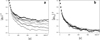 |
Fig. 4 (a) Correlation functions |g E |2 vs. |ε| for six different metapixels of size 96 × 96 px. (b) Correlation function for homogeneous illumination as computed from (11). |
 |
Fig. 5 Relative error on the determination of the value of the TMFP as a function of the metapixel size. |
4.3 Characterization of an heterogeneous system
To illustrate the potential of the technique, we have applied it to a more complex sample that we designed using beads of two different sizes. The beads were placed in a cell of thickness 25 mm and with an illuminated glass surface of 8 cm× 10 cm. To prepare a simple phantom, we divided the measuring cell in halves with a wall and separately filled both parts with the beads of mentioned diameters. Then the wall was carefully removed in a way that the border between different beads stack remained sufficiently sharp. Figure 6a shows the speckle pattern corresponding to the two sub-parts of the image. Figure 6b shows the spatially resolved map of the l* distribution. The size of the zone on which every value of l* is measured is chosen here to be 32 × 32 pixels. Despite the poor detailing obtained with a low-resolution InGaAs detector, the border between the locations of the beads with different diameters is very explicit and the values of l* corresponds to the predicted ones with a good accuracy.
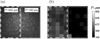 |
Fig. 6 (a) The observed speckle pattern for a sample made of two different materials. The dotted and dashed zones correspond to two different beads diameters, and hence to two different values of l*. (b) Extracted values of l*. The size of each square is 32 × 32 pixels, corresponding to 7.5 × 7.5 mm on the sample. |
5 Conclusions
We presented a method to measure transport mean free path l* based on the use of a cheap tunable laser source. The scattered intensity correlation function with the incident wavelength modulation is measured using a multi-speckle setup. The method allows probing samples in non-destructive way, simple and cost-effective in its arrangement and fast in data processing. Interestingly, we demonstrated that it can be readily modified in a way to provide spatially resolved measurements and, thus, can be applied for the measurements in non-homogeneous samples. The statistical noise may be reduced if the size of the matrix of the detecting camera is increased, or by performing another kind of ensemble average. The method has been demonstrated here with a near-IR DFB laser, but may be easily performed with 760 or 780 nm chip which allow the use of visible camera. Alternate laser source may also be gas laser with an adjustable cavity length, or an optical parametric oscillator.
Author contribution statement
J.C. provided the idea of measuring the transport mean free path with wavelength variations and supervised the work. A.M., J.C. and J.F. designed the experiments. A.M. carried out the experiments. J.F. and A.M. made the theoretical analysis of experimental data. All authors participated to the redaction of the manuscript.
Acknowledgments
The authors acknowledge the ESA for the postdoctoral financial support of A.M. and J.C. acknowledges the ANR (ANR-16-CE30-0022) and CNRS for funding. We thank Hervé Tabuteau and Valérie Marchi for helping us to prepare PDMS samples, Patrick Chales for the help with the data acquisition and Axelle Amon for scientific discussions.
Appendix
The method of the static transmission consists in measuring the total transmitted optical power through the sample. This method allows the measurement of transport mean free path without the use of any reference sample with known scattering mean free path. The sample is a parallel slab of thickness L that was illuminated with a focused light beam with wavelength of 1556 nm. The scattered transmitted light was measured using an InGaAs photodiode (OSI Optoelectronics, FCI-InGaAs-1000). In order to diminish the electronic noise, the beam was mechanically chopped, and measurements were done using a lock-in detection. The transmitted scattered intensity was measured in directions making different angles with respect to the output normal of the slab. From those measurements, the total transmitted intensity was obtained. The incident intensity was obtained by focussing the beam on the photodiode.
The transmission through a scattering slab is [36]: (A.1)with
  . This result is obtained for a model point source of diffusing light located at a distance z
0 behind the illuminated face of the slab. For PDMS, the absorption length is l
a
= 27.7 mm [38],
. This result is obtained for a model point source of diffusing light located at a distance z
0 behind the illuminated face of the slab. For PDMS, the absorption length is l
a
= 27.7 mm [38],  [31] and we take
  . The thickness being known, the value of l* may be obtained from the value of the transmission T. The relative uncertainty on transmission is obtained with repeated experiments and is 4%, leading to a relative uncertainty on l* of 5%.
References
- A. Ishimaru, Wave Propagation and Scattering in Random Media (Academic Press, 1978) [Google Scholar]
- L.V. Wang, H.-I. Wu, Biomedical optics: principles and imaging (John Wiley & Sons, 2012) [Google Scholar]
- S.T. Flock, M.S. Patterson, B.C. Wilson, D.R. Wyman, IEEE Trans. Biomed. Eng. 36 , 1162 (1989) [Google Scholar]
- C. Baravian, F. Caton, J. Dillet, J. Mougel, Phys. Rev. E 71 , 066603 (2005) [Google Scholar]
- F. Caton, C. Baravian, J. Mougel, Opt. Express 15 , 2847 (2007) [PubMed] [Google Scholar]
- M. Heckmeier, G. Maret, Europhys. Lett. 34 , 257 (1996) [Google Scholar]
- B.W. Pogue, M.S. Patterson, Phys. Med. Biol. 39 , 1157 (1994) [CrossRef] [PubMed] [Google Scholar]
- M.Q. Brewster, Y. Yamada, Int. J. Heat Mass Transf. 38 , 2569 (1995) [Google Scholar]
- E. Gratton, S. Fantini, M.A. Franceschini, G. Gratton, M. Fabiani, Philos. Trans. Roy. Soc. B: Biol. Sci. 352 , 727 (1997) [CrossRef] [Google Scholar]
- D.A. Boas, D.H. Brooks, E.L. Miller, C.A. DiMarzio, M. Kilmer, R.J. Gaudette, Q. Zhang, IEEE Sig. Process. Mag. 18 , 57 (2001) [CrossRef] [Google Scholar]
- S.L. Jacques, B.W. Pogue, J. Biomed. Opt. 13 , 041302 (2008) [CrossRef] [PubMed] [Google Scholar]
- A.H. Hielscher, H.K. Kim, L.D. Montejo, S. Blaschke, U.J. Netz, P.A. Zwaka, G. Illing, G.A. Muller, J. Beuthan, IEEE Trans. Med. Imag. 30 , 1725 (2011) [CrossRef] [Google Scholar]
- W. Brown (Ed.), Dynamic Light Scattering: The Method and Some Applications (Oxford University Press, 1993) [Google Scholar]
- B.J. Berne, R. Pecora, Dynamic Light Scattering With Applications to Chemistry (Dover Publication Inc., 2000) [Google Scholar]
- W. Leutz, J. Riča, Opt. Commun. 126 , 260 (1996) [Google Scholar]
- G. Maret, P.E. Wolf, Z. Phys. B 65 , 409 (1987) [CrossRef] [Google Scholar]
- D.J. Pine, D.A. Weitz, J.X. Zhu, E. Herbolzheimer, J. Phys. France 51 , 2101 (1990) [CrossRef] [EDP Sciences] [Google Scholar]
- D.A. Weitz, D.J. Pine, Diffusing-wave spectroscopy, in Dynamic Light Scattering: The Method and Some Applications , edited by W. Brown (Oxford University Press, 1993), pp. 652–720 [Google Scholar]
- R.C. Haskell, L.O. Svaasand, T.-T. Tsay, T.-C. Feng, B.J. Tromberg, M.S. McAdams, J. Opt. Soc. Am. A 11 , 2727 (1994) [Google Scholar]
- D.J. Cuccia et al., J. Biomed. Opt. 14 , 14 (2009) [Google Scholar]
- F. Scheffold, I.D. Block, Opt. Express 20 , 192 (2012) [PubMed] [Google Scholar]
- C.M. Aegerter, G. Maret, Prog. Opt. 52 , 1 (2009) [CrossRef] [Google Scholar]
- J.H. Li, A.A. Lisyansky, T.D. Cheung, D. Livdan, A.Z. Genack, Europhys. Lett. 22 , 675 (1993) [Google Scholar]
- J.M. Drake, A.Z. Genack, Phys. Rev. Lett. 63 , 259 (1989) [CrossRef] [PubMed] [Google Scholar]
- A.Z. Genack, J.M. Drake, Europhys. Lett. 11 , 331 (1990) [Google Scholar]
- V. Toronov, E. D'Amico, D. Hueber, E. Gratton, B. Barbieri, A. Webb, Opt. Express 11 , 2717 (2003) [PubMed] [Google Scholar]
- H.K. Kim, U.J. Netz, J. Beuthan, A.H. Hielscher, Opt. Express 16 , 18082 (2008) [PubMed] [Google Scholar]
- S. Panigrahi, J. Fade, H. Ramachandran, M. Alouini, Opt. Exp. 24 , 16066 (2016) [CrossRef] [Google Scholar]
- A.Z. Genack, Fluctuations, correlation and average transport of electromagnetic radiation in random media, in Scattering And Localization Of Classical Waves In Random Media. Series: Series on Directions in Condensed Matter Physics , edited by P. Sheng (World Scientific, Singapore, 1990), pp. 207–311 [CrossRef] [Google Scholar]
- J. Crassous, M. Erpelding, A. Amon, Phys. Rev. Lett. 103 , 013903 (2009) [CrossRef] [PubMed] [Google Scholar]
- D.J. Vera, M.U. Durian, Phys. Rev. E 53 , 3215 (1996) [Google Scholar]
- M. Ghijsen, B. Choi, A.J. Durkin, S. Gioux, B.J. Tromberg, Biomed. Opt. Express 7, 870 (2016) [CrossRef] [PubMed] [Google Scholar]
- N. George, A. Jain, Appl. Phys. 4 , 201 (1974) [CrossRef] [Google Scholar]
- H. Fujii, T. Asakura, Y. Shindo, J. Opt. Soc. Am. 66 , 1217 (1976) [Google Scholar]
- D.J. Pine, D.A. Weitz, G. Maret, P.E. Wolf, E. Herbolzheomer, P.M. Chaikin, Scattering and localization of classical waves in random media, in Dynamical Correlations of Multiply Scattered Light , edited by P. Sheng (World Scientific, Singapore, 1990), pp. 312–372 [Google Scholar]
- I.M. Vellekoop, P. Lodahl, A. Lagendijk, Phys. Rev. E 71 , 056604 (2005) [Google Scholar]
- F. Ayers, A. Grant, D. Kuo, D.J. Cuccia, A.J. Durkin, Proc. SPIE 6870 , 07–1 (2008) [Google Scholar]
- M.R. Querry et al., Optical constants of minerals and other materials from the millimeter to the UV. US Army Rep. CRDEC-CR-88009, Aberdeen, MD, 1987 [Google Scholar]
- J. Crassous, Eur. Phys. J. E 23 , 145 (2007) [CrossRef] [EDP Sciences] [Google Scholar]
Cite this article as: Alesya Mikhailovskaya, Julien Fade, Jérôme Crassous, Speckle decorrelation with wavelength shift as a simple way to image transport mean free path, Eur. Phys. J. Appl. Phys. 85, 30701 (2019)
All Figures
|
Fig. 1 (a) Schematic view of the light propagation inside a highly diffusing material. (b) Boundary condition for the density of photons inside the material. The beam behaves as a point source located at a distance z 0 inside the material, and the density of photons extrapolates to 0 at a distance ze outside the material. |
| In the text | |
|
Fig. 2 Experimental set-up: (1) DFB laser, (2) expanding lens, (3) sample slab, (4) infrared camera, (5) objective lens, (6) diaphragm. |
| In the text | |
|
Fig. 3 Decorrelation of the scattered intensity with the wavelength modulation of the incident light for the samples of TiO2 particles embedded in PDMS matrix. Symbols stand for the experimental points and the lines correspond to the fitting curves obtained from equation (8): blue circles − “turbid slab”, black squares − “white slab”. |
| In the text | |
|
Fig. 4 (a) Correlation functions |g E |2 vs. |ε| for six different metapixels of size 96 × 96 px. (b) Correlation function for homogeneous illumination as computed from (11). |
| In the text | |
|
Fig. 5 Relative error on the determination of the value of the TMFP as a function of the metapixel size. |
| In the text | |
|
Fig. 6 (a) The observed speckle pattern for a sample made of two different materials. The dotted and dashed zones correspond to two different beads diameters, and hence to two different values of l*. (b) Extracted values of l*. The size of each square is 32 × 32 pixels, corresponding to 7.5 × 7.5 mm on the sample. |
| In the text | |
Current usage metrics show cumulative count of Article Views (full-text article views including HTML views, PDF and ePub downloads, according to the available data) and Abstracts Views on Vision4Press platform.
Data correspond to usage on the plateform after 2015. The current usage metrics is available 48-96 hours after online publication and is updated daily on week days.
Initial download of the metrics may take a while.