| Issue |
Eur. Phys. J. Appl. Phys.
Volume 85, Number 2, February2019
Electrical Engineering Symposium (SGE 2018)
|
|
|---|---|---|
| Article Number | 20902 | |
| Number of page(s) | 9 | |
| Section | Physics of Energy Transfer, Conversion and Storage | |
| DOI | https://doi.org/10.1051/epjap/2019180300 | |
| Published online | 08 March 2019 | |
https://doi.org/10.1051/epjap/2019180300
Regular Article
An analysis of power losses in nanocrystalline and thin-gauge non-oriented SiFe materials for application to high-speed electrical machines★
1
Univ. Grenoble Alpes, CNRS, Grenoble INP, G2Elab, 38000 Grenoble, France
2
Moving Magnet Technologies SA, 25000 Besançon, France
* e-mail: This email address is being protected from spambots. You need JavaScript enabled to view it.
Received:
7
October
2018
Received in final form:
6
December
2018
Accepted:
31
January
2019
Published online: 8 March 2019
Abstract
In this paper, the potential of thin sheet SiFe NO20 and nanocrystalline materials for the realization of the magnetic circuit of high-speed machines is analyzed in a complete procedure. Firstly, intrinsic properties of materials are precisely characterized. Next, the original and a modified model of Bertotti are applied for the modeling of power losses. These models are then used to predict losses in a simplified test bench which simulates the magnetic core of a real machine. FEM simulations in Altair FLUX 2D and experimental measurements are respectively carried out and results obtained show a good agreement leading to the confirmation of the potential of materials and the validation of the realized procedure.
Contribution to the Topical issue “Electrical Engineering Symposium (SGE 2018)”, edited by Adel Razek.
© A.-T. Vo et al., EDP Sciences, 2019
 This is an Open Access article distributed under the terms of the Creative Commons Attribution License (http://creativecommons.org/licenses/by/4.0), which permits unrestricted use, distribution, and reproduction in any medium, provided the original work is properly cited.
1 Introduction
High-speed electrical machines are getting more attention, the main challenge in their realization is that some physical effects play no role at low speeds but become significant at high speeds with powers of several kilowatts [1]. One of the most apparent effects is the redistribution of power losses between magnetic, mechanical and aerodynamic components. This requires designers to consider multi-physics models that meet strict requirements in the fields of magnetism, thermodynamics and mechanics [2].
In this article, power losses analysis in high-speed applications is made. We focus exclusively on the modeling of iron losses component because of its rapid growth with the operation frequency of machines. At high speed, it represents a substantial part of the total losses of machines. To reduce iron losses means actually to significantly increase machine efficiency. Moreover, by pushing iron losses estimation to a better accuracy from the design phase, we can optimize the geometry of machines in order to have the best possible performance. Accordingly, our study consists of evaluating the possibilities of using low iron losses grade soft magnetic materials for the realization of the magnetic circuit of high-speed machines.
Two materials are envisaged: non-oriented SiFe NO20 sheets and nanocrystalline ribbons having respectively thickness of 0.2 mm and 25 μm.
The NOXX material is a type of thin non-oriented FeSi sheets having a silicon content of 2–3% and a thickness varies from 0.1 to 0.3 mm. The name of material specifies the thickness of sheets, we will study the NO20 and thus sheets having thickness of 0.2 mm. These low sheet thicknesses induce significantly lower dynamic losses and these materials are therefore exploited at much higher frequencies than the grid frequency [3].
The second material, nanocrystalline, is in the form of ribbon and is even less conventional. The nanocrystallines are characterized by a biphasic microstructure with very small grains, typically less than 50 nm, in an amorphous matrix. They have the advantage of having very low magnetic losses because of their small thickness (typically 25 μm) and their high resistivity, about three times greater than that of SiFe steels. Nanocrystalline materials can be an interesting solution for high frequency applications [4,5]. A major disadvantage of these materials is their mechanical fragility, which creates difficulties in assembly processes of the magnetic circuits of machines [6].
In order to estimate the potential of these materials in high speed machine applications, we propose a complete and relevant analysis including their magnetic characterization, the identification of their iron loss models and the validation of these models by numerical simulations and experiments. Concerning the magnetic losses, numerous available models in the literature can be classified in three groups [7]:
-
models based on the Steinmetz equation [8];
-
models separating magnetic losses into static and dynamic losses, and with or without consideration of magnetic domains structure and processes of magnetization [9,10];
 (1)
(1)
In several studies [9,14], Bertotti showed that the modeling of magnetic losses by considering only the first two components of equation (1) was not sufficiently precise. As a result, the excess loss term has been proposed. He justified the origin of this component by statistical considerations and physically interpreted its property according to microscopic constants characterizing material.
The proportionality coefficients of the Bertotti model depend on properties of material under consideration and are identified by curve fitting techniques from experimental data. We present in the third part of this paper a complete identification procedure of these coefficients.
Finally, finite element simulations in Altair FLUX 2D and experiments carried out on a simplified device developed by the Moving Magnet Technologies company allow us to validate the accuracy of the loss models of each material under operating conditions similar to those of real machines.
2 Intrinsic characterization
2.1 Studied samples
Two samples are used for the intrinsic characterization of nanocrystalline material: a wound torus (Nano-1), and a stacked torus (Nano-2), both have the same inner and outer diameter (24 × 29 mm). They belong to NANOPHY grade of Aperam group1 and have undergone a conventional annealing of nano-crystallization.
The thin sheet NO20 is characterized by using two samples: a standardized Epstein type (NO20-1) supplied by ArcelorMittal and a stacked torus (NO20-2) with the dimension of 24 × 28 mm. Figure 1 shows the different configurations envisaged.
2.2 Magnetic measurements
The identification of Bertotti's iron loss models requires measured losses while induction is imposed in sinusoidal at different amplitudes and frequencies. To do this, we use a modular numerical characterization bench consisting of an amplifier allowing the excitation of the samples, a current sensor to evaluate the magnetic field and a voltage sensor to evaluate the magnetic flux (so the induction).
The measurements range of amplitude and frequency of each sample is specified in Table 1. The amplitude goes up to a value very close to the saturation of the samples and the frequency reaches sufficiently high values to guarantee the accuracy of the models of magnetic losses over a wide frequency range. In order to ensure the accuracy of the Bertotti models, the correct sinusoidal shape of the induction must be ensured for all measurements. European standard EN60404 recommends adjusting the form factor of the secondary side voltage, i.e. the derivative of induction, to 1.111 ± 1%. This condition is fulfilled by the use of a digital waveform controller developed at our laboratory [16].
Summary of characterization results.
2.3 Characterization result
We measured the centered hysteresis curves of the four samples at different induction and frequency values. For instance, Figure 2 shows the results obtained at 1 T and 1 kHz. Nanocrystallines are more permeable, but saturate faster than NO20. The area of the nanocrystalline hysteresis cycles are much thinner than those of NO20. Magnetic losses of samples at high frequencies are shown in Figures 3 (NO20) and 4 (Nano). For the same level of induction and frequency, the magnetic losses of nanocrystalline are 40–60 times lower than those of NO20 (see Tab. 1).
These figures also clearly show the influence of cutting, in the case of Nano-2 and NO20-2 stacked cores. This cutting was performed by EDM in the case of NO20 or by laser in the case of nanocrystalline. It significantly reduces permeability and increases losses. Although they are less traumatic than punching [17,18], these cutting methods degrade the materials significantly.
For all measured points, the form factor of the induction respects the standard IEC 60404.
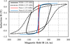 |
Fig. 2 Hysteresis curves of samples at 1 T−1 kHz. |
 |
Fig. 3 Magnetic losses of NO20 at high frequency. |
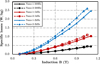 |
Fig. 4 Magnetic losses of nanocrystalline at high frequency. |
3 Identification of magnetic loss models
The identification of loss models is carried out for these four samples.
3.1 Bertotti's loss models
Equation (1) calculating the magnetic losses as a function of frequency and peak induction is valid only if B(t) is in sinusoidal form. This formula has been generalized to apply for any waveform by introducing the time derivative dB/dt as expressed in equation (2) [9]. This method, named (M1), has been available in Altair FLUX software for transient magnetic regime calculations. (2)
(2)
In order to apply this model, the skin effect must be negligible. Furthermore, in [19,20], the excess coefficient k exc is reported to increase rapidly with the peak induction, however for practical use and especially when implemented in finite element software, it is assumed to be constant. Consequently, although we identify k hys , k eddy and k exc with data obtained at different frequencies and levels of induction, the model (M1) has a low accuracy at high induction peak and high frequency.
In Altair FLUX, users can modify all exponential coefficients, this action actually implies the dependence of proportional coefficients on frequency and induction peak allowing a higher prediction accuracy. The adapted model (M2) has the following form. (3)
(3)
For the rest, each sample is modeled by these two models of Bertotti (M1) and (M2) which will be compared in terms of accuracy.
3.2 Identification of loss models
The coefficient of each term of the Bertotti's loss models can be found theoretically using macroscopic and microscopic constants. However, these constants strongly depend on structure and chemical composition of material and are not obviously accessible. We therefore use a purely mathematical identification approach consisting of an optimization problem as illustrated in Figure 5 and whose purpose is to minimize the difference between measurement values and values derived from the model.
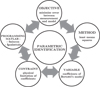 |
Fig. 5 Parametric identification approach. |
3.2.1 Formation of the problem
The least mean squares method is used to express the objective function written in the form of equation (4):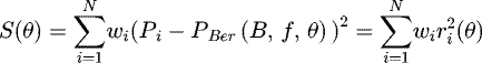 (4)where r
i
(θ) are the absolute deviations or errors between the measurement and the prediction, θ represents the variables to be identified, w
i
is interpreted as the weighting factor of each measurement. We also present here the notion of relative error: r
i% = 100r
i
/P
i
.
(4)where r
i
(θ) are the absolute deviations or errors between the measurement and the prediction, θ represents the variables to be identified, w
i
is interpreted as the weighting factor of each measurement. We also present here the notion of relative error: r
i% = 100r
i
/P
i
.
For data whose measurement noise is Gaussian, we do not consider w
i
, and we simply put w
i
= 1 [21]. However, this is not our case, using w
i
= 1 the optimization program always tries to minimize the absolute error at points with the largest losses corresponding to high frequency and high induction measurements. For this reason, the optimization program creates a very large relative error for low frequency losses curves. This problem can be solved by adding a weighting factors so that  . The objective function currently represents the sum of the relative errors. Any operating point P (B, f) has the same importance in this function. This also implies that the model precision at high induction is sacrificed for the one at low induction. However, in most electrical machine applications, high induction is used to minimize the amount of material used. In addition, losses at low induction can be considered negligible. Finally, in order to exploit the advantage of two types of weighting factor, we decide to implement a Pareto-type multi-criteria optimization. The principle of Pareto optimization is to look for several solutions of multi-objective problems and then build the boundary that consists of the dominant points (visible in Fig. 6).
The quality of identification is evaluated by the normalized quadratic means of residuals from each model in the form of equation (5).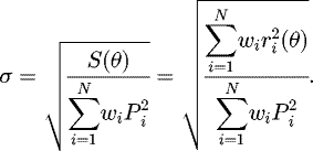 (5)
(5)
The two evaluation criteria for optimization are therefore:
-
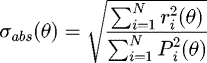 : the normalized quadratic means of absolute residual (%);
 -
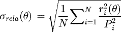 : the normalized quadratic means of relative residual (%).
The identification objectives are fixed at: 
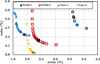 |
Fig. 6 Pareto front corresponding to the original model (M1) of the samples. |
3.2.2 Identification strategy
For the original Bertotti model (M1), in the absence of a significant skin effect, k
eddy
varies a priori very slightly around its predetermined value by the conductivity σ and the thickness d of material. On the other hand, the other coefficients are constrained to not being negative:
For the modified model (M2), the coefficients never vary simultaneously but one after the other according to the sequence α exc → α hys → β hys → α eddy in order to preserve as much as possible the physical meaning of the loss models. The order chosen corresponds to the inverse order of certainty of the coefficients. Indeed, the coefficient related to the eddy current losses is well known and it has the lowest level of uncertainty, while the coefficient of excess losses is the most difficult to determine because of its higher level of uncertainty.
Whatever their values, the coefficients are all bounded: 0 < α hys , β hys , α eddy , α exc ≤ 4. The upper bound is experimentally limited to 4 because the greater the exponential coefficient, the more the loss model is sensitive to the uncertainties of measurements. Finally, for a fully modified mathematical Bertotti model, we have 7 variables to determine.
3.2.3 Programming of the identification program
The identification program is written under MATLAB® using the function fgoalattain () [22]. This function makes it possible to find local minima of multi-objective problems by using the successive quadratic optimization algorithm. By identifying the parameters of Bertotti's original model (M1), it was realized that the relative errors were too high, especially for samples whose iron losses increase rapidly at high induction. In order to ensure the robustness of the identification process, the points of high induction are removed from the database.
3.2.4 Identification results
The set of identification results is summarized in Table 2. The original model (M1) is valid for a lower induction range than that of the modified model (M2). For nanocrystalline samples, even if the high induction points are eliminated (limit at 1.0 T), the original model (M1) cannot adapt to the measured data, so the exponential coefficient α exc must be varied. For the modified model (M2), all the coefficients are varied while remaining within the imposed limits [0,4] and the evaluation criteria adapt well to the predefined values (<5%).
Figures 7 and 8 shows an example of the iron losses curves and the difference of two models compared to measured data in the case of the NO20-1 sample. The difference in performance between two models is found at the induction higher than 1.3 T.
Identification result of two Bertotti's loss models for all samples.
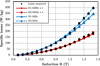 |
Fig. 7 Comparison of measured data and results from both models in the case of NO20-1 at 5 Hz and 2 kHz (M1: original Bertotti model, M2: modified Bertotti model). |
 |
Fig. 8 Relative difference between results of the two models and measured data in the case of NO20-1. |
4 Validation bench for calculating magnetic losses
4.1 Working principle of the bench
In order to test and validate the models, we rely on an experimental device developed by the company MMT which allows to test magnetic circuits of simple shapes in conditions close to their actual use in electric machines.
The principle is to rotate a surface-placed permanent magnet rotor (5 pairs of poles) in a stator constituted by the magnetic circuit to be tested, which may be a smooth or slotted core. This stator is connected in pivot linkage with the frame of the bench. The power that the stator transmits to the frame corresponds to the iron losses and the aerodynamic losses. Figure 9 shows a view of the assembly.
The power balance transmitted by the rotor is given by: (6)
with P
mec
the mechanical output power of the rotor, P
fer
the magnetic losses of the stator, P
aero
the aerodynamic losses.
(6)
with P
mec
the mechanical output power of the rotor, P
fer
the magnetic losses of the stator, P
aero
the aerodynamic losses.
The force sensor was chosen to measure the rotor torque. The mechanical power is calculated by: (7)
d, the lever arm, is equal to 4 mm. Ω is the rotational speed. The measured torque Fd accuracy is of the order of ten μNm.
(7)
d, the lever arm, is equal to 4 mm. Ω is the rotational speed. The measured torque Fd accuracy is of the order of ten μNm.
Aerodynamic losses are estimated using equation (9) proposed by Vrancik in [23] (8)where l and r respectively represent the length and the outside diameter, ρ
air
is the density of air, C
d
represents the coefficient of surface friction. This last coefficient is calculated empirically using the following equation:
(8)where l and r respectively represent the length and the outside diameter, ρ
air
is the density of air, C
d
represents the coefficient of surface friction. This last coefficient is calculated empirically using the following equation: (9)with Re the Reynolds number:
 (10)and δ the thickness of the gap, υ the kinematic viscosity of air.
The rotation of the magnet is carried out by a variable and adjustable speed drive motor. Under the effect of a supply of compressed air, the inlet turbine is rotated and drives the output shaft through an oil bearing. The rotation speed can reach 100,000 rpm.
In this study, two slot-less cores stacked in NO20 and annealed nanocrystalline were tested and simulated. The geometry of the magnetic part including the magnets and the core is illustrated in Figure 15a. The geometrical parameters of the core studied are given in Table 3.
The finite element simulations are carried out in Altair FLUX 2D. Both spatial components of the flux density vector, corresponding to major and minor axes of B-locus shape, are taken into account for the iron losses calculation performed in a postprocessor mode.
 |
Fig. 9 Set-up of validation bench and a zoom on magnetic parts. |
Characteristics of core and magnets.
4.2 Experimental results
Figure 10 illustrates the mechanical power curves for each cores, aerodynamic losses and estimated iron losses of the NO20 core. As indicated in Table 3, the variation of geometry of the cores is considered negligible, the aerodynamic losses are therefore as the same order of magnitude, a single curve is drawn.
It is realized that the share of aerodynamic losses in the total mechanical power of the torus NO20 increases as a function of the speed of rotation and becomes non-negligible in the procedure for calculating iron losses. The iron losses of the NO20 core seem reasonable. On the other hand, there is obviously an error in the case of the nanocrystalline. The mechanical losses corresponding to the sum of the iron losses and the aerodynamic losses of this material are lower than the aerodynamic losses, whatever the frequency considered. The iron losses of the nanocrystallines core would therefore be negative. Two reasons are mentioned to explain this inconsistent result: either the formula of the dynamic loss estimation is not enough accuracy, or the measurements with the nanocrystalline core are not good.
Indeed, as indicated in the part 2 of the article, iron losses of nanocrystalline samples are particularly low (40–60 times lower than those of NO20 samples). The measured mechanical losses must, therefore, logically be very close to the estimated values of aeronautical losses; However, it is not the case. It can be assumed that equation (9) overestimated the aerodynamic losses. In order to solve this, it is envisaged to carry out measurements with a plastic core to eliminate the iron losses of the material and thus obtain experimental values of aerodynamic losses. Nevertheless, if this reason is proved to be the correct one, it is necessary to recalculate also the iron losses of the NO20 with the good values of aerodynamic losses.
On the other hand, the measurements on the Nano core are very delicate, the standard deviations observed in this case are very high as shown in Figure 14. They are greater than 100% compared to the measured average value. These measurements are not repeatable because the force sensor used is no longer suitable.
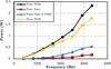 |
Fig. 10 Experimental results of measurements. |
4.3 Comparison simulation and experimentation
Figure 11 compares the simulation results with those of the experimental ones, including the aerodynamic losses, obtained in the case of the NO20 core. It shows that the simulations are going in the right direction. More precisely, the (M1) and (M2) models give very similar results with a difference of less than 5%. This last result is explained by the fact that the magnetic excitation created by the magnets is weak resulting in a relatively low induction in the cores. The distribution of induction in the NO20 core is illustrated in Figure 15b. The maximum value of the peak induction is about 0.8 T and most of the toroid surface has a very low peak induction, less than 0.2 T. At this induction level, there is no remarkable difference between the two models.
The NO20-1 data estimate well low frequency losses but underestimate them at high frequency. In the case of NO20-2, it's totally the opposite. However, for both cases, the measurement results agree well with the standard deviation of the measurements as shown in Figure 12. For the nanocrystalline core, simulation and experimentation do not correspond for the reasons mentioned above as found in Figure 13.
 |
Fig. 11 Comparison between measurement results and simulation results in the case of the NO20 core. |
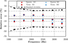 |
Fig. 12 Comparison of the error resulting from two models and the standard deviation of the measurements in the case of NO20 core. |
 |
Fig. 13 Comparison between the measurement results and the simulation results in the case of the nanocrystalline core. |
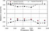 |
Fig. 14 Comparison of the error resulting from two models and the standard deviation of the measurements in the case of nanocrystalline core. |
 |
Fig. 15 (a) Simulated geometry in Altair FLUX of the experimental device, (b) distribution of the maximum value of the B module over an electrical period in the stator. |
5 Conclusions
In this study, we proposed an approach running from the intrinsic characterization of material to the estimation of iron losses in a magnetic circuit through modeling, simulation and a validation model. The tested materials NO20 and nanocrystalline are interesting for high frequency applications. We have shown the influence of the cutting and the advantage of nanocrystalline (50 times fewer iron losses than the NO20). The estimation of the losses of the device by the original model (M1) and the modified model (M2) of Bertotti are very close considering the weak operating inductions. The comparison of simulated and measured losses in the case of NO20 core validates the proposed approach. In the case of the nanocrystalline core, further investigations are necessary.
In order to increase the precision of the measurements, in the next studies, we envisage:
-
to use magnets whose remanent magnetization is higher to increase the level of peak induction in cores and therefore the level of iron losses;
-
to use a force sensor with finer precision;
-
to measure aerodynamic losses experimentally.
Acknowledgments
We would like to thank Mr. Adrien GILSON, engineer at MMT for his contribution to the experimental validation bench.
Author contribution statement
Anh-Tuan Vo: Conducted the experimental measurements from intrinsic to validation level, performed the analysis and wrote the paper. Marylin Fassenet: Performed the numerical simulation, planned experiments and helped supervise the project. Laure Arbenz: Conceived the validation test bench and helped supervise the project. Afef Kedous-Lebouc: Supervised the project and verified all performed analysis. Christophe Espanet: Supervised the project, contributed analysis tool, helped on preparation of samples. All authors provided critical feedback and helped shape the research, analysis and manuscript.
References
- A. Tenconi, S. Vaschetto, A. Vigliani, IEEE Trans. Ind. Electr. 61 , 3022 (2014) [CrossRef] [Google Scholar]
- P. Pfister, Y. Perriard, IEEE Trans. Ind. Electr. 57 , 296 (2010) [CrossRef] [Google Scholar]
- A. Krings, A. Boglietti, A. Cavagnino, S. Sprague, IEEE Trans. Ind. Electr. 64 , 2405 (2017) [CrossRef] [Google Scholar]
- K. Praveena, K. Sadhana, S. Bharadwaj, S.R. Murthy, J. Magn. Magn. Mater. 321 , 2433 (2009) [Google Scholar]
- W. Shen, F. Wang, D. Boroyevich, C. Wesley Tipton IV, IEEE Trans. Ind. Appl. 44 , 213 (2008) [Google Scholar]
- A. Kedous-Lebouc, Matériaux magnétiques en Génie Elec-trique 1 & 2 (Hermès-Lavoisier, 2006) [Google Scholar]
- A. Krings, J. Soulard, J. Electr. Eng. 10 , 162 (2010) [Google Scholar]
- C.P. Steinmetz, Trans. Am. Inst. Electr. Eng. IX, 1 (1892) [CrossRef] [Google Scholar]
- G. Bertotti, IEEE Trans. Magn. 24 , 621 (1988) [Google Scholar]
- F. Fiorillo, A. Novikov, IEEE Trans. Magn. 26 , 2904 (1990) [Google Scholar]
- D.C. Jiles, D.L. Atherton, J. Magn. Magn. Mater. 61 , 48 (1986) [Google Scholar]
- D.C. Jiles, J.B. Thoelke, M.K. Devine, IEEE Trans. Magn. 28 , 27 (1992) [Google Scholar]
- T. Chevalier, A. Kedous-Lebouc, B. Cornut, C. Cester, Physica B 275 , 197 (2000) [CrossRef] [Google Scholar]
- G. Bertotti, J. Appl. Phys. 57 , 2110 (1985) [Google Scholar]
- S. Tumanski, Handbook of Magnetic Measurements (CRC Press, 2016) [CrossRef] [Google Scholar]
- A.-T. Vo, M. Fassenet, A. Kedous-Lebouc, F. Blache, M.-P. Vaillant, C. Boudinet, Novel model-based digital controller for facilitating soft magnetic materials measurement under controlled excitations, in 15th International Workshop on 1&2 Dimensional Magnetic Measurement and Testing, Grenoble, France , 2018 [Google Scholar]
- A. Kedous-Lebouc, B. Cornut, J.C. Perrier, P. Manfé, T. Chevalier, J. Magn. Magn. Mater. 254–255 , 124 (2003) [Google Scholar]
- A. Kedous-Lebouc, O. Messal, A. Youmssi, J. Magn. Magn. Mater. 426 , 658 (2017) [Google Scholar]
- G. Bertotti, Hysteresis in Magnetism: For Physicists, Materials Scientists, and Engineers (Academic Press, 1998) [Google Scholar]
- E. Barbisio, F. Fiorillo, C. Ragusa, IEEE Trans. Magn. 40 , 1810 (2004) [Google Scholar]
- H.J. Motulsky, L.A. Ransnas, FASEB J. 1 , 365 (1987) [CrossRef] [PubMed] [Google Scholar]
- F. Gembicki, Y. Haimes, IEEE Trans. Autom. Cont. 20 , 769 (1975) [CrossRef] [Google Scholar]
- J.E. Vrancik, Prediction of windage power loss in alternators (National Aeronautics and Space Administration, USA, 1971) [Google Scholar]
ArcelorMittal, “Data sheet Nanocristalline cores Nanophy.”
Cite this article as: Anh-Tuan Vo, Marylin Fassenet, Laure Arbenz, Afef Kedous-Lebouc, Christophe Espanet, An analysis of power losses in nanocrystalline and thin-gauge non-oriented SiFe materials for application to high-speed electrical machines, Eur. Phys. J. Appl. Phys. 85, 20902 (2019)
All Tables
All Figures
 |
Fig. 1 Closed magnetic circuit configurations used for the characterization [15]. |
| In the text | |
|
Fig. 2 Hysteresis curves of samples at 1 T−1 kHz. |
| In the text | |
|
Fig. 3 Magnetic losses of NO20 at high frequency. |
| In the text | |
|
Fig. 4 Magnetic losses of nanocrystalline at high frequency. |
| In the text | |
|
Fig. 5 Parametric identification approach. |
| In the text | |
|
Fig. 6 Pareto front corresponding to the original model (M1) of the samples. |
| In the text | |
|
Fig. 7 Comparison of measured data and results from both models in the case of NO20-1 at 5 Hz and 2 kHz (M1: original Bertotti model, M2: modified Bertotti model). |
| In the text | |
|
Fig. 8 Relative difference between results of the two models and measured data in the case of NO20-1. |
| In the text | |
|
Fig. 9 Set-up of validation bench and a zoom on magnetic parts. |
| In the text | |
|
Fig. 10 Experimental results of measurements. |
| In the text | |
|
Fig. 11 Comparison between measurement results and simulation results in the case of the NO20 core. |
| In the text | |
|
Fig. 12 Comparison of the error resulting from two models and the standard deviation of the measurements in the case of NO20 core. |
| In the text | |
|
Fig. 13 Comparison between the measurement results and the simulation results in the case of the nanocrystalline core. |
| In the text | |
|
Fig. 14 Comparison of the error resulting from two models and the standard deviation of the measurements in the case of nanocrystalline core. |
| In the text | |
|
Fig. 15 (a) Simulated geometry in Altair FLUX of the experimental device, (b) distribution of the maximum value of the B module over an electrical period in the stator. |
| In the text | |
Current usage metrics show cumulative count of Article Views (full-text article views including HTML views, PDF and ePub downloads, according to the available data) and Abstracts Views on Vision4Press platform.
Data correspond to usage on the plateform after 2015. The current usage metrics is available 48-96 hours after online publication and is updated daily on week days.
Initial download of the metrics may take a while.