| Issue |
Eur. Phys. J. Appl. Phys.
Volume 83, Number 3, September 2018
|
|
|---|---|---|
| Article Number | 30904 | |
| Number of page(s) | 6 | |
| Section | Physics of Energy Transfer, Conversion and Storage | |
| DOI | https://doi.org/10.1051/epjap/2018180079 | |
| Published online | 06 November 2018 | |
https://doi.org/10.1051/epjap/2018180079
Regular Article
An analytical model for the magnetostriction strain of ferromagnetic materials subjected to multiaxial stress
GeePs − Group of Electrical Engineering − Paris, UMR CNRS 8507, CentraleSupélec, Univ. Paris-Sud, Université Paris-Saclay, Sorbonne Université, 3 rue Joliot-Curie, Plateau de Moulon,
91192
Gif-sur-Yvette Cedex, France
* e-mail: This email address is being protected from spambots. You need JavaScript enabled to view it.
Received:
2
February
2018
Received in final form:
23
May
2018
Accepted:
26
June
2018
Published online: 6 November 2018
Abstract
Magnetostriction is the magnetisation-induced strain in ferromagnetic materials. It highly depends on mechanical stress. Stress state in electromagnetic devices is usually multiaxial and its effect on magnetostrictive properties is not easily predicted. In this paper, an original three-parameter analytical model for the stress-dependent magnetostriction strain of ferromagnetic materials is proposed. It is based on a simplified energetic description of magneto-elastic behaviour. It follows a similar method previously adopted for the description of the effect of stress on the magnetic permeability of magnetic materials. It is applied for the first time to the magnetostriction behaviour and results in a simple formula to express the effect of multiaxial magneto-mechanical loadings on the magnetostriction strain. The approach also naturally includes the description of the so-called ΔE effect. The analytical formula is derived in the paper. It shows very satisfying agreement with experimental results on iron–cobalt alloy and pure iron specimen.
© L. Daniel, published by EDP Sciences, 2018
 This is an Open Access article distributed under the terms of the Creative Commons Attribution License (http://creativecommons.org/licenses/by/4.0), which permits unrestricted use, distribution, and reproduction in any medium, provided the original work is properly cited.
1 Introduction
Magnetic and mechanical behaviours are strongly coupled [1]. Magnetisation is very sensitive to the application of stress, leading to significant effects on the performance of electromagnetic devices [2–4]. Conversely, the magnetisation process is associated with a mechanical deformation called magnetostriction. Magnetostriction can be used for actuation purposes, for instance using giant magnetostrictive materials [5–7]. It is also one of the origins of the noise emitted by electromagnetic devices such as transformers [8–10]. Magnetostriction itself is known to be sensitive to stress [11–14]. Although very significant, this effect of stress on the magnetostriction strain is rarely taken into account in the modelling of electromagnetic devices or limited to uniaxial configurations where the stress is uniaxial and applied in the direction parallel to the applied magnetic field [15–17]. However, stress state in electromagnetic devices is usually multiaxial, making the 1D approaches irrelevant. Recently, 3D magneto-mechanical models for the prediction of the magnetostriction strain have been proposed. Some of them are based on the definition of the magneto-elastic free energy of the material [18–20]. These approaches can handle full 3D configurations, but the number of parameters required for the modelling can be high and their identification can be tedious. Some others are based on a multiscale description of magneto-elastic couplings [21–27]. These models provides a very useful insight into magneto-elastic coupling effects, but they are usually too complex to be directly implemented into numerical analysis tools. In order to overcome this issue, simplified approaches have been derived from these full multiscale approaches [28]. These simplifications lead to a loss of information, notably regarding internal heterogeneity effects, but can be implemented into structural analysis tools for electromagnetic devices [29–31]. In this paper, the simplification procedures are extended further so as to obtain a fully analytical model for the magnetostriction strain as a function of applied magnetic field and stress. It follows a similar method previously adopted for the description of the effect of stress on the magnetic permeability of magnetic materials [32]. In Section 2, the simplified 3D magneto-elastic model [28] is recalled. It is shown in Section 3 how further simplifications can provide a fully analytical definition for the stress-dependent magnetostriction strain. The magnetostriction strain under particular loadings is then detailed (Sect. 4) and a parameter identification method is proposed (Sect. 5). Section 6 is finally dedicated to an illustration of the model prediction and to the comparison to experimental results.
2 Simplified magneto-elastic model
A magneto-elastic constitutive law can be derived from the description of a magnetic material as a set of magnetic domains with known magnetisation (Ms) and random orientation [28]. This approach, detailed in reference [28] is recalled hereafter. The local free energy (Eq. (1)) of a magnetic domain k is expressed as the sum of three contributions:
 (1)
(1)
The Zeeman energy  (Eq. (2)) introduces the effect of the applied magnetic field on the equilibrium state. μ0 is the vacuum permeability. Hk and Mk are the magnetic field and magnetisation in the magnetic domain.
 (2)
(2)
The elastic energy  (Eq. (3)) introduces the effect of stress on the magnetic equilibrium. σ is the applied stress and
  is the magnetostriction strain in the magnetic domain. Like the other energy terms, this energy is defined except for a constant. The derivation of equation (3) from the classical definition of the elastic energy is detailed in reference [24].
 (3)
(3)
Macroscopic anisotropy can be described through an anisotropy energy term  added to the free energy. Equation (4) gives this additional term for a uniaxial anisotropy along direction v, with K the anisotropy constant. If we assume macroscopic isotropy, this term vanishes:
 (4)
(4)
Such an approach, very close to Armstrong model [22], was proposed in reference [29] in the 2D case. For a three-dimensional configuration and considering isotropic and isochoric magnetostriction [28], the following definitions for the local magnetisation Mk and magnetostriction strain  are used:
 (5)
(5)
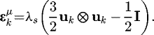 (6)
(6)
Ms is the saturation magnetisation of the material, uk is the orientation of the magnetisation in the domain k, λs is the saturation magnetostriction constant and I the second-order identity tensor. Note that equation (6) corresponds to isochoric magnetostriction ( ), so that volume magnetostriction, occurring for high magnetic field levels, is neglected.
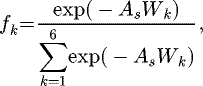
The magneto-elastic behaviour is obtained by defining the volume fraction fk of a domain with orientation uk through the use of a Boltzmann probability function [21]:
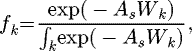 (7)
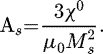
where As is a material parameter linked to the initial anhysteretic susceptibility χ0 [24]:
(7)
where As is a material parameter linked to the initial anhysteretic susceptibility χ0 [24]:
 (8)Once the probability fk is defined, the macroscopic magnetisation M and magnetostriction ϵμ are obtained, thanks to an averaging operation over all possible directions:
 (9)
(9)
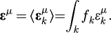 (10)This integration step can be performed numerically using a discretisation of possible orientations uk [25].
Although simplified compared to the full multiscale model [25], this approach is not analytical. Integration operations are required in equations (7), (9) and (10). It can be made analytical by considering a further simplified configuration with a limited number of domains. This is expected to aggravate the limitations of the model proposed in reference [28], particularly in the case of complex anisotropies or high level of heterogeneity. However, such a strategy was already successfully applied in reference [33] for the definition of an equivalent stress for magnetic behaviour, in reference [34] to describe the effect of plasticity on the magnetic behaviour, or in reference [32] to derive an analytical expression for the stress-dependent magnetic permeability of ferromagnetic materials. It is developed here to derive an original analytical expression for the stress-dependent magnetostriction strain.
3 Stress-dependent magnetostriction strain
We consider a homogeneous isotropic magnetic material subjected to a magnetic field H in the direction x (H = Hx) in an orthonormal coordinate system (O,x,y,z). This material is simultaneously subjected to a multiaxial stress state σ given by equation (11):
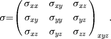 (11)
Any relative orientation between the applied magnetic field and the principal stress can be described. Following the approach proposed in reference [32], the material equilibrium state can be defined using a simplified energy description. The material is assumed to be divided into six domains noted k (k={1, 2, 3, 4, 5, 6}) with magnetisation oriented along uk (uk={ x, −x, y, −y, z, −z }). Each domain k is characterised by its free energy (Eq. (12)) obtained after simplification of equation (1). For strongly anisotropic media, an anisotropy term (e.g. Eq. (4)) should be kept in the free energy (Eq. (12)), to the price of a complexification of the analytical expressions obtained.
(11)
Any relative orientation between the applied magnetic field and the principal stress can be described. Following the approach proposed in reference [32], the material equilibrium state can be defined using a simplified energy description. The material is assumed to be divided into six domains noted k (k={1, 2, 3, 4, 5, 6}) with magnetisation oriented along uk (uk={ x, −x, y, −y, z, −z }). Each domain k is characterised by its free energy (Eq. (12)) obtained after simplification of equation (1). For strongly anisotropic media, an anisotropy term (e.g. Eq. (4)) should be kept in the free energy (Eq. (12)), to the price of a complexification of the analytical expressions obtained.
 (12)Under these assumptions, the free energy for each domain k can be explicitly written. The volume fraction fk of each domain (Eq. (7)) is then estimated from equation (13) using a discrete summation. The relative weight for a given orientation k is directly related to the relative energy of this orientation compared to the other orientations.
 (13)which leads to
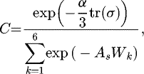
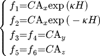 (14)using the following notations:
 (15)
(15)
 (16)
(16)
 (17)
(17)
 (18)As shown in reference [32], the material magnetisation M is obtained, thanks to the discrete summation (Eq. (19)), which leads to the analytical definition (Eq. (20)) for the magnetisation:
 (19)
(19)
 (20)This expression introduces the saturation magnetisation Ms of the material and two additional constants α and κ. Due to the form of the magnetostriction tensor (Eq. (6)), only the components σxx, σyy and σzz appear in the analytical expression of the magnetisation (Eq. (20)) − see the expression of the magneto-elastic energy in equation (3).
Similarly, the magnetostriction strain is defined by the discrete summation (Eq. (21)):
 (21)
(21)
It is easily shown that it can be written in the form
 (22)
with
(22)
with
 (23)Under the considered assumptions (isotropic homogeneous material), equation (23) provides an analytical expression for the magnetostriction strain of the material under any multiaxial stress state, with any orientation with respect to the magnetic field. Three material parameters are introduced: the saturation magnetostriction λs and two additional parameters κ and α. These parameters are related to standard material parameters by equations (16)–(18).
4 Particular configurations
Further simplifications can be obtained if less complex loadings are considered. The corresponding expressions are given hereafter:
-
From equation (23), it is verified that under no applied stress nor magnetic field, the magnetostriction strain is zero. It is also verified that when the magnetic field is getting very high, λ tends towards λs.
-
If no stress is applied, the magnetostriction strain reduces to equation (24):
 (24)
(24)
-
If no magnetic field is applied, the magnetostriction strain reduces to equation (25):
 (25)
(25)
-
The magnetostriction strain under uniaxial stress and no applied field is given by equation (26). This expression describes the so-called ΔE effect [35,36]:
 (26)
(26)
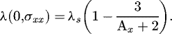
-
If we consider a uniaxial stress σxx in the direction x, equation (23) reduces to
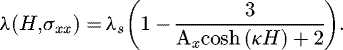 (27)
(27)
5 Identification of parameters κ and α
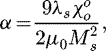
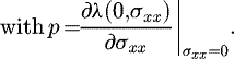
The proposed model is based on three material parameters (λs, κ and α). λs is the maximum magnetostriction strain and its significance is clear. As defined in reference [32], κ can be identified from the initial anhysteretic susceptibility  of the material under no applied stress (Eq. (28)). This relation is obtained by combining equations (17) and (18). The parameter α can be identified from equation (29), obtained by combining equations (16) and (18). α can also be extracted from a ΔE measurement curve. The ΔE effect is the loss of linearity in the stress–strain curve of magnetic materials [35] (see Sect. 5). It is due to the magnetostriction strain that superimposes to the elastic strain. This magnetostriction strain under no applied field, and for a uniaxial stress, is given by equation (26). By considering the initial slope p of the ΔE curve, the parameter α can be obtained (Eq. (30)):
 (28)
(28)
 (29)
(29)
 (30)
(30)
 (31)
(31)
6 Model prediction
The proposed model (Eq. (23)) can provide a prediction of the magnetostriction strain of an isotropic material for any magneto-mechanical loading, i.e. for any magnetic field H and any stress tensor σ, whatever the relative orientation between them. It must be noticed that the model describes the anhysteretic behaviour, so that hysteresis effects are not included in the proposed description. As an example, Figure 1 shows the evolution of the magnetostriction strain under no applied magnetic field as a function of stress under uniaxial, equibiaxial, hydrostatic and pure shear stress states. These stress states are, respectively, defined by a diagonal stress tensor with the values (σ, 0, 0), (σ, σ, 0), (σ, σ, σ) and (σ, −σ, 0) on the diagonal. The magnetostriction strain is measured along the direction x.
The results show very similar evolution as those obtained for the magnetic susceptibility in reference [32]. It is worth noting that an applied hydrostatic stress has no effect on the magnetic susceptibility, which is consistent with the fact that magnetostriction strain is isochoric (trace (ϵμ) = 0). The uniaxial stress curve (u) corresponds to the description of the ΔE effect, as defined in reference [35].
Very few measurements are available in the literature for an experimental validation under complex loadings. Most of the available data are restricted to uniaxial configurations for which the stress is applied in the direction parallel to the magnetic field. Here, the model has been compared to magnetostriction strain measurements under uniaxial stress presented in reference [36] for an iron–cobalt alloy. They consist of anhysteretic measurements on flat samples of dimensions 2.5 × 12.5 × 110 mm3 loaded along the longest direction. The strain was measured using strain gages. Numerical simulations performed on a geometry corresponding to the experimental setup have shown that the form effect (deformation due to the magnetic forces on the specimen [37]) has little effect on the strain measurement area, so that the presented data reflect the magnetostriction strain. Figures 2 and 3 show the strain measurements, respectively, parallel and perpendicular to the magnetic field direction for various stress levels. The material parameters have been identified as λs = 5810−6, κ = 2.210−3 m/A and α = 10−7 Pa−1. The left side of the figure shows the prediction of the proposed model, and the right side shows the experimental results. Regarding the modelling results, the definition of the magnetostriction curve (Eq. (27)) incorporates naturally the ΔE effect, which is the magnetostriction strain as a function of stress under no applied field. In order to be consistent with the representation of experimental results, this initial strain has been removed in the representation of modelling results. The plotted numerical results are then defined as λ = λ(H, σxx) − λ(0, σxx).
Considering the simplicity of the model (only Eq. (27) is used), Figures 2 and 3 show a very satisfactory agreement between experimental and modelling results. The model tends to slightly overestimate the longitudinal strain. On the contrary, the transverse strain is underestimated by the model. Since an isotropic approach has been used for the material, the predicted transverse strain is simply half the longitudinal strain with an opposite sign. The experimental results do not show a similar ratio, suggesting an initial anisotropy is not taken into account in the model. The agreement could probably be enhanced by introducing additional material parameters, notably to describe initial anisotropy effects.
Another experimental validation can be made based on the measurement of the ΔE effect. The ΔE effect is an apparent dependency of the Young's modulus to the stress level when a tensile or compressive test is performed on a magnetic specimen [1]. It is a manifestation of the effect of stress on the magnetostriction strain (under no applied magnetic field) [35]. Indeed, the application of stress modifies the magnetic domain structure and hence generates a magnetostriction strain. This magnetostriction strain is superimposed on the elastic strain, so the stress–strain curve obtained from a tension or compression test is non-linear. A description of the ΔE effect based on this interpretation has been thoroughly discussed in reference [35]. The modelling approach presented in this paper describes the ΔE effect through equation (26). The results have been plotted in Figures 4 and 5for an iron-cobalt alloy (different from the alloy presented in Figs. 2 and 3) and for pure iron, respectively. The experimental results are simply extracted from reference [35]. The experimental setup is the same as the one used for Figures 2 and 3. The results from the model proposed in reference [35] are also reproduced with a dotted line.
It can be seen that both models and experimental results exhibit very satisfying agreement, both in trends and values. Only two parameters are required for the proposed modelling of the ΔE effect since the parameter κ is used only under applied magnetic field. The modelling results from reference [35] have simply been reproduced. In particular, the material parameters, deduced from single crystal data, have not been changed. It is clear that the modelling of the ΔE effect (dotted lines) could be improved by fitting the modelling parameters to the experimental data. On the contrary, the modelling parameters used in the present approach (Eq. (26)) have been adjusted to the experimental data, which explains the slightly better agreement observed. The main difference between the two modelling approaches is that the description proposed in reference [35] is predictive (in the sense that material parameters can be deduced from the basic properties of single crystals) but restricted to the case where no magnetic field is applied. On the contrary, the present model is more phenomenological (in the sense that the material parameters have to be fitted on macroscopic measurements) but also more general in the sense that it can combine the application of stress and magnetic field (see Figs. 2 and 3). It can again be observed that the measured transverse strain is not half the longitudinal strain in amplitude, contrarily to the hypothesis made in both models. This can be attributed to anisotropy effects not taken into account in the modelling approaches.
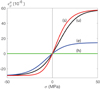 |
Fig. 1 Magnetostriction strain (maximum principal strain) under no applied magnetic field as a function of stress intensity for uniaxial (u), equibiaxial (e), hydrostatic (h) and pure shear (s) stress states (modelling parameters: λs = 5810−6, κ = 2.210−3 m/A, α = 10−7 Pa−1). |
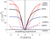 |
Fig. 2 Longitudinal magnetostriction strain under uniaxial stress for an iron–cobalt alloy: analytical model (left) and experimental results from reference [36] (right) (modelling parameters: λs = 5810−6, κ = 2.210−3 m/A, α = 10−7 Pa−1). |
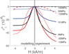 |
Fig. 3 Transverse magnetostriction strain under uniaxial stress for an iron–cobalt alloy: analytical model (left) and experimental results from reference [36] (right) (modelling parameters: λs = 5810−6, κ = 2.210−3 m/A, α = 10−7 Pa−1). |
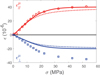 |
Fig. 4 ΔE effect for an iron–cobalt alloy: longitudinal and transverse magnetostriction strain as a function of the applied stress σ (uniaxial), modelling (lines) and experimental (points) results from reference [35]. The dotted line reproduces the modelling results obtained in reference [35]. The plain line shows the results from equation (26) (modelling parameters: λs = 4010−6, α = 1.2510−7 Pa−1). |
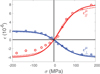 |
Fig. 5 ΔE effect for pure iron: longitudinal and transverse magnetostriction strain as a function of the applied stress σ (uniaxial), modelling (lines) and experimental (points) results from reference [35]. The dotted line reproduces the modelling results obtained in reference [35]. The plain line shows the results from equation (26) (modelling parameters: λs = 810−6, α = 2.410−8 Pa−1). |
7 Conclusion
In this paper, an original analytical model for the definition of the stress-dependent magnetostriction strain of magnetic materials is proposed. It is based on a very simplified description of the energetic equilibrium underlying magnetic behaviour. The approach results in a simple formula to express the effect of multiaxial magneto-mechanical loadings on the magnetostriction strain. The multiaxiality of stress is naturally introduced in this approach, and no assumption is made on the relative orientation between stress and magnetic field. Only three materials parameters are required to describe this complex magneto-mechanical behaviour. The three parameters can be, respectively, identified from an anhysteretic curve under no applied stress, a magnetostriction curve under no applied stress and a ΔE effect measurement. They can also be fitted from experimental results under stress. This analytical model can be useful for electromagnetic design when users require the implementation of a magnetostriction model into standard structural analysis tools. Due to the strong assumptions made in the construction of the model, it is expected that limitations will be found in cases of strong anisotropy or high heterogeneities.
References
- B.D. Cullity, C.D. Graham, Introduction to Magnetic Materials, 2nd edn (John Wiley & Sons, Inc., New York, 2009) [Google Scholar]
- N. Takahashi, H. Morimoto, Y. Yunoki, D. Miyagi, J. Magn. Magn. Mater. 320, e925 (2008) [Google Scholar]
- H. Ebrahimi, Y. Gao, H. Dozono, K. Muramatsu, T. Okitsu, D. Matsuhashi, IEEE Trans. Magn. 52, 8201404 (2016) [Google Scholar]
- K. Yamazaki, H. Takeuchi, IEEE Trans. Ind. Appl. 53, 963 (2017) [Google Scholar]
- F. Claeyssen, N. Lhermet, R. Le Letty, P. Bouchilloux, J. Alloys Compd. 258, 61 (1997) [Google Scholar]
- G. Engdahl, Handbook of Giant Magnetostrictive Materials (Academic Press, Cambridge, UK, 2000) [Google Scholar]
- A.G. Olabi, A. Grunwald, Mater. Des. 29, 469 (2008) [Google Scholar]
- A.J. Moses, IEEE Trans. Magn. 10, 154 (1974) [Google Scholar]
- B. Weiser, H. Pfutzner, J. Anger, IEEE Trans. Magn. 36, 3759 (2000) [Google Scholar]
- Y.H. Chang, C.H. Hsu, H.L. Chu, C.P. Tseng, IEEE Trans. Magn. 47, 2780 (2011) [Google Scholar]
- R.M. Bozorth, Ferromagnetism (Van Norstand, New York, 1951) [Google Scholar]
- P.I. Anderson, A.J. Moses, H.J. Stanbury, IEEE Trans. Magn. 43, 3467 (2007) [Google Scholar]
- Y. Kai, Y. Tsuchida, T. Todaka, M. Enokizono, IEEE Trans. Magn. 50, 6786404 (2014) [Google Scholar]
- A. Belahcen, D. Singh, P. Rasilo, F. Martin, S.G. Ghalamestani, L. Vandevelde, IEEE Trans. Magn. 51, 2001204 (2015) [Google Scholar]
- M.J. Sablik, D.C. Jiles, IEEE Trans. Magn. 29, 2113 (1993) [Google Scholar]
- O. Bottauscio, A. Lovisolo, P.E. Roccato, M. Zucca, C. Sasso, R. Bonin, IEEE Trans. Magn. 44, 3009 (2008) [Google Scholar]
- H. El Bidweihy, E. Della Torre, Y. Jin, L.H. Bennett, M. Ghahremani, IEEE Trans. Magn. 48, 3360 (2012) [Google Scholar]
- L. Hirsinger, G. Barbier, C. Gourdin, R. Billardon, Mech. Electromagn. Mater. Struct. 19, 54 (2000) [Google Scholar]
- K. Fonteyn, A. Belahcen, R. Kouhia, P. Rasilo, A. Arkkio, IEEE Trans. Magn. 46, 2923 (2010) [Google Scholar]
- P. Rasilo, D. Singh, U. Aydin, F. Martin, R. Kouhia, A. Belahcen, A. Arkkio, IEEE Trans. Magn. 52, 7300204 (2016) [Google Scholar]
- N. Buiron, L. Hirsinger, R. Billardon, J. Phys. IV 9, 187 (1999) [Google Scholar]
- W.D. Armstrong, J. Appl. Phys. 91, 2202 (2002) [Google Scholar]
- L. Daniel, O. Hubert, R. Billardon, Comput. Appl. Math. 23, 285 (2004) [Google Scholar]
- L. Daniel, O. Hubert, N. Buiron, R. Billardon, J. Mech. Phys. Solids 56, 1018 (2008) [Google Scholar]
- L. Daniel, N. Galopin, Eur. Phys. J. Appl. Phys. 42, 153 (2008) [CrossRef] [EDP Sciences] [Google Scholar]
- L. Daniel, M. Rekik, O. Hubert, Arch. Appl. Mech. 84, 1307 (2014) [CrossRef] [Google Scholar]
- D. Vanoost, S. Steentjes, J. Peuteman, G. Gielen, H. De Gersem, D. Pissoort, K. Hameyer, J. Magn. Magn. Mater. 414, 168 (2016) [Google Scholar]
- L. Daniel, O. Hubert, M. Rekik, IEEE Trans. Magn. 51, 7300704 (2015) [Google Scholar]
- L. Bernard, X. Mininger, L. Daniel, G. Krebs, F. Bouillault, M. Gabsi, IEEE Trans. Magn. 47, 2171 (2011) [Google Scholar]
- L. Bernard, L. Daniel, IEEE Trans. Magn. 51, 7002513 (2015) [Google Scholar]
- M. Liu, O. Hubert, X. Mininger, F. Bouillault, L. Bernard, IEEE Trans. Magn. 52, 8000212 (2016) [Google Scholar]
- L. Daniel, IEEE Trans. Magn. 49, 2037 (2013) [Google Scholar]
- O. Hubert, L. Daniel, J. Magn. Magn. Mater. 323, 1766 (2011) [Google Scholar]
- O. Hubert, S. Lazreg, IEEE Trans. Magn. 48, 1277 (2012) [Google Scholar]
- L. Daniel, O. Hubert, Eur. Phys. J. Appl. Phys. 45, 31101 (2009) [CrossRef] [EDP Sciences] [Google Scholar]
- O. Hubert, L. Daniel, IEEE Trans. Magn. 46, 401 (2010) [Google Scholar]
- L. Hirsinger, R. Billardon, IEEE Trans. Magn. 31, 1877 (1995) [Google Scholar]
Cite this article as: Laurent Daniel, An analytical model for the magnetostriction strain of ferromagnetic materials subjected to multiaxial stress, Eur. Phys. J. Appl. Phys. 83, 30904 (2018)
All Figures
|
Fig. 1 Magnetostriction strain (maximum principal strain) under no applied magnetic field as a function of stress intensity for uniaxial (u), equibiaxial (e), hydrostatic (h) and pure shear (s) stress states (modelling parameters: λs = 5810−6, κ = 2.210−3 m/A, α = 10−7 Pa−1). |
| In the text | |
|
Fig. 2 Longitudinal magnetostriction strain under uniaxial stress for an iron–cobalt alloy: analytical model (left) and experimental results from reference [36] (right) (modelling parameters: λs = 5810−6, κ = 2.210−3 m/A, α = 10−7 Pa−1). |
| In the text | |
|
Fig. 3 Transverse magnetostriction strain under uniaxial stress for an iron–cobalt alloy: analytical model (left) and experimental results from reference [36] (right) (modelling parameters: λs = 5810−6, κ = 2.210−3 m/A, α = 10−7 Pa−1). |
| In the text | |
|
Fig. 4 ΔE effect for an iron–cobalt alloy: longitudinal and transverse magnetostriction strain as a function of the applied stress σ (uniaxial), modelling (lines) and experimental (points) results from reference [35]. The dotted line reproduces the modelling results obtained in reference [35]. The plain line shows the results from equation (26) (modelling parameters: λs = 4010−6, α = 1.2510−7 Pa−1). |
| In the text | |
|
Fig. 5 ΔE effect for pure iron: longitudinal and transverse magnetostriction strain as a function of the applied stress σ (uniaxial), modelling (lines) and experimental (points) results from reference [35]. The dotted line reproduces the modelling results obtained in reference [35]. The plain line shows the results from equation (26) (modelling parameters: λs = 810−6, α = 2.410−8 Pa−1). |
| In the text | |
Current usage metrics show cumulative count of Article Views (full-text article views including HTML views, PDF and ePub downloads, according to the available data) and Abstracts Views on Vision4Press platform.
Data correspond to usage on the plateform after 2015. The current usage metrics is available 48-96 hours after online publication and is updated daily on week days.
Initial download of the metrics may take a while.