© S. Dufour and G. Vinsard, published by EDP Sciences, 2018

1 Introduction

One of the main types of shape memory alloys (SMA) is nickel–titanium (NiTi). It is used in various applications such as actuators [1]. However, the actuation frequency is low. To overcome this limitation, body heating with eddy current is investigated.

The general operating principle of the SMA is as follows. At low temperatures, the alloy is in its martensitic state. A mechanical constraint is applied to distort the piece permanently. If this metal is then heated beyond its transformation temperature, it changes from martensitic to austenitic state. Provided the deformation does not include folds with too low curvature, the alloy comes back to its initial state (Fig. 1).

The main factor of the process is the heating time or cooling time to change phase. Joule heating is a good candidate to decrease the heating time [2]. The induction heating has been evaluated for wires, as well as tubes in torsion and recently considered in the case of beams [3] but only in the case of small deformations (i.e. with linear strain-displacement equations).

A complete mechanical model requires semi-empirical data during the phase change: the control of the rise of temperature with respect to the time as well as its spatial homogeneity is important to determine numerically the phase of the alloy.

Here, the aim of the paper is to use a flexible model of computation of induced currents to study the sensitivity of the different parameters (beam geometry, frequency, decentring) for a given shape. The change of shape is included in the case of large deformations (the linear strain-displacement equations are then no longer valid).

To leave the full mechanical model aside, the deformation of the beam is given as a function of time with the help of the well-known elastica model [4]. It allows us to compute the induced currents and the temperature for each given shape as a function of time.

Fig. 1 Ni-Ti Beam functioning. Top panel: time start for induction heating, middle panel: beyond the transformation temperature, bottom panel: end of the heating.

2 Geometric parameterization of the change of shape

The mechanical assumption is that the parametric equation of the beam (Fig. 1) is the one of the elastica [5]: 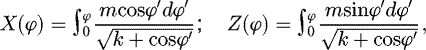$$X(\phi )={\int }_0^{\phi }\frac{m\cos {\phi }^{\prime }d{\phi }^{\prime }}{\sqrt{k+\cos {\phi }^{\prime }}};Z(\phi )={\int }_0^{\phi }\frac{m\sin {\phi }^{\prime }d{\phi }^{\prime }}{\sqrt{k+\cos {\phi }^{\prime }}}\text{,}$$(1) where φ ∈ [ − ψ, ψ]. ψ is determined by the constraint that the beam length is constant: 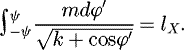$${\int }_{-\psi }^{\psi }\frac{md{\varphi }^{\prime }}{\sqrt{k+\cos {\varphi }^{\prime }}}=l_X\text{,}$$(2)This parametric equation comes from the elasticity of a beam in large deformation [4]. Briefly, if a cantilever beam (Fig. 2) is considered (i.e. the beam is fixed at one side and a force F_n is normally applied at the other side), the deflection equation is as follows: $$EI\frac{d^2\theta }{d{s}^2}=-F_n\cos (\theta -{\theta }_f)\text{,}$$(3)where θ is the tangent angle with respect to the horizontal axis, E is the Young's modulus, I the bending moment of inertia, s the curvilinear abscissa, and θ_f is the value of the angle θ at the end side.

Then, equation (3) after integration becomes $$\frac{d\theta }{ds}=\sqrt{\frac{2F_n}{EI}}\sqrt{\sin ({\theta }_{\max }-{\theta }_f)-\sin (\theta -{\theta }_f)}\text{,}$$(4) where θ_max is such that ${\displaystyle \dot{\theta }}(s)=0$ (Fig. 2). Equation (1) can be found with 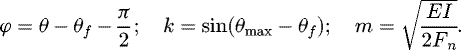$$\varphi =\theta -{\theta }_f-\frac{\pi }{2};k=\sin ({\theta }_{\max }-{\theta }_f);m=\sqrt{\frac{EI}{2F_n}}\text{.}$$(5)

The same deflection is obtained if the fixed end is replaced by a symmetric axis.

It has been experimentally noticed on top of Figure 1 that the distorted beam has globally the shape of an elastica, which corresponds to a relaxation of the elasticity stress tensor after a plastic deformation (see Fig. 2 when F_n decreases).

The change of shape during the heating is taken into account by using the elastica parameterization (Eq. (1)): the decrement of parameter k allows continuously following the change of shape, from the initial shape obtained after relaxation to the final plane original form (corresponding to k → − 1).

Fig. 2 Cantilever beam for two different forces Fn.

3 Computational model

3.1 Eddy current computation

The beam region is defined as a domain D of the Euclidean space E₃. To find a position X in this domain, an application Φ is built such that any X corresponds to x in a reference space $D$ with Φ(x) = X.

The coordinates (relative to the frame vectors (k_x, k_y, k_z)) in the space E₃ being given in vector form, we define the map L as 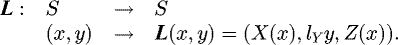$$\begin{array}{llll}L:\hfill & S\hfill & \to \hfill & S\hfill \\ \hfill & (x,y)\hfill & \to \hfill & L(x,y)=(X(x),l_{Y}y,Z(x)).\hfill \end{array}$$(6) The arguments (x, y) of L lie in the subset $S=[-\psi ,\psi ]\times [-1/\mathrm{2,1}/2]$ of a dimensionless space where ψ satisfies the length constraint (Eq. (2)) and the transverse length is l_y. (X, Z) are the functions (Eq. (1)) where m is a fixed value (0.02) and k is the parameter that allows the change of shape. The image of S by L is labelled S.

The normal N to this surface is used to build the application $$\mathrm{\Phi }(x)=L(x,y)+HzN(x,y)=X$$(7) between x = (x, y, z) and X = (X, Y, Z). H is the height of the beam. And the beam region, noted D, is the image $\mathrm{\Phi }(D)$, where $D=S\times [-1/\mathrm{2,1}/2]$ is the dimensionless space of reference.

Different formulations can be used to compute eddy currents. The chosen one is a T − Ω formulation, since it allows to treat only the beam (and not the surrounding domain). The relative permeability of Ni-Ti being 1.002, it is approximated to 1. The T − Ω equations for conducting domain D are as follows: $$\nabla \times \left(\nabla \times T\right)-\frac{2j}{{\delta }^2}\left(T-\nabla \mathrm{\Omega }-H_s\right)=0\text{in}D\text{.}$$(8) $$\nabla \cdot T=0\text{in}D\text{.}$$(9) $$\nabla \cdot \left({\mu }_0\left(T-\nabla \Omega \right)\right)=0\text{in}{E}_3\text{.}$$(10) T vanishes outside D. δ is the skin depth (δ ≃ 1.4 mm at 100 kHz for the Ni-Ti). H_s the magnetic induction source field (of the inductor). It is obtained by a Biot–Savart computation. 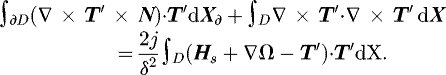T is solution of the weak form: $${\int }_{\partial D}\left(\nabla \times T\times N\right)·\mathrm{d}{X}_{\partial }+{\int }_D\nabla \times T\cdot \nabla \times \mathrm{d}X=\frac{2j}{{\delta }^2}{\int }_D(H_s+\nabla \mathrm{\Omega }-T)·\mathrm{T}\mathrm{d}\mathrm{X}\mathrm{e}\mathrm{.}$$(11)

The boundary integral obtained in the weak form by the integration by parts vanishes due to the condition T × N = 0. ∇ ⋅ T reduces to the jump of T ⋅ N on ∂D, since T is free divergence in D and vanishes outside D. Ω is defined in the whole space. Since the permeability is μ₀, to avoid considering the outer mesh of the beam, Ω is computed with the Biot–Savart formula: 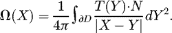$$\Omega (X)=\frac{1}{4\pi }{\int }_{\partial D}\frac{T(Y)N}{|X-Y|}d{Y}^2.$$(12)

Equations (11) and (12) are coupled equations.

As the geometry is evolutionary, the remeshing is necessary. For simplicity reasons, an alternative Lagrangian approach is chosen, where the computation of T by equation (11) is done in the space of reference $D$, at the cost of a more complex expression of the differential operators.

The change of coordinates is done with the parameterization (Eq. (7)). In summary, the following table can be displayed:

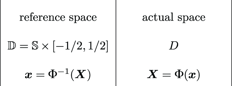
The electric and magnetic potentials (T, Ω) in D become (t, ω) in $D$, where $$T(X)=\nabla \mathrm{\Phi }(x)t(x)\Omega (X)=\omega (x)\text{.}$$(13) In the same way, $$H_s=(X)=\nabla \mathrm{\Phi }(x)h_s(x)N=\nabla \mathrm{\Phi }(x){\displaystyle \overrightarrow{n}}\text{,}$$(14)where n is in the reference space (0, 0, 1/H). The Gram matrix g is introduced as 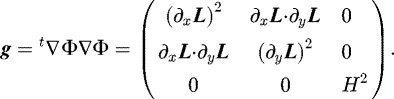$$g={}^{\mathit{t}}\nabla \mathrm{\Phi }\nabla \mathrm{\Phi }=\left(\begin{array}{ccc}\hfill {({\partial }_{x}L)}^2\hfill & \hfill {\partial }_{x}L\cdot {\partial }_{y}L\hfill & \hfill 0\hfill \\ \hfill {\partial }_{x}L\cdot {\partial }_{y}L\hfill & \hfill {({\partial }_{y}L)}^2\hfill & \hfill 0\hfill \\ \hfill 0\hfill & \hfill 0\hfill & \hfill H^2\hfill \end{array}\right)\text{.}$$(15)

The Gram determinant is $$|g{|}^{1/2}=H|{\partial }_{x}L\times {\partial }_{y}L|\text{.}$$(16)

For a beam of small thickness with respect to the skin depth (here H ∼ δ/10), the main component of T is directed along the normal N, and its variation with respect to N is low. Then, the electric potential vector t can reasonably be approximated by $$t(x)t(x,y)n\text{.}$$(17) With the transforms,

equation (11) becomes $${\int }_{S}H(g^{-1}\nabla t)\cdot \nabla t|g{|}^{1/2}dxdy=\frac{2j}{{\delta }^2}{\int }_S\left(H{h}_s\cdot n+\frac{1}{H^2}{\partial }_z\omega -\frac{t}{H}\right)t^{\prime }|g{|}^{1/2}dxdy\text{,}$$(18) where the source term h_s ⋅ n is n(∇ Φ(x))⁻¹ ⋅ H_s i.e. (H_s ⋅ N). Equation (12) is computed by a Biot–Savart-like integral as the unique contribution of t to the computation of ω is the jump of t on the upper and lower boundaries of the domain $D$. w is computed as follows: $$w(x)=\frac{1}{4\pi }{\int }_S\frac{t(x^{\prime },y^{\prime })|g(x^{\prime },y^{\prime },1/2){|}^{1/2}}{|\mathrm{\Phi }(x)-\mathrm{\Phi }(x^{\prime },y^{\prime },1/2)|}d{x}^{\prime }d{y}^{\prime }-\frac{1}{4\pi }{\int }_S\frac{t(x^{\prime },y^{\prime })|g(x^{\prime },y^{\prime },-1/2){|}^{1/2}}{|\mathrm{\Phi }(x)-\mathrm{\Phi }(x^{\prime },y^{\prime },-1/2)|}d{x}^{\prime }d{y}^{\prime }\text{.}$$(19)

Equation (19) contains singularities, and truncation errors appear due to the proximity of the upper and lower boundaries. Then, a specific analytic treatment is set up to compute with enough accuracy w and its derivative with respect to z.

To avoid the resolution of a linear system with a non-sparse matrix (the CPU time of a LU decomposition rises as the number of nodes cubed), the computation of t and ∂_zω is alternated: equation (18) is computed for a given ∂_zω, and ∂_zω is computed again with equation (19). It allows to get a convergence for a limited number of iterations. The parallel solver MUMPS (MUltifrontal Massively Parallel Sparse direct Solver) is used to reduce the computation time.

3.2 Joule power and thermal model

The source field h_s is obtained by Biot–Savart's formula. Joule power losses can be computed after solving the eddy current problem as $$P_j={\int }_S\frac{H}{\sigma }(g^{-1}\nabla t)\cdot \nabla t^{*}|g{|}^{1/2}dxdy\text{,}$$(20) with its associated resistance R and power density ${\displaystyle \dot{q}}$ ( t^* is the conjugate of t). The electric conductivity σ depends on the temperature (1.21 MS/m in the martensitic state and 1.31 MS/m in the austenitic state).

The Fourier number is about 250 for the normal direction to the beam, but 0.25 for the tangential directions, which means that the temperature is almost independent of this normal direction, but that the transient temperature distribution has to be considered in $S$. If, at time t the temperature is labelled θⁿ and at time t + Δt as θⁿ⁺¹, the variational form of the heat equation is obtained in $S$ as $$\forall {\theta }^{\prime }{\int }_S\frac{\rho C_p}{\mathrm{\Delta }t}({\theta }^{n+1}-{\theta }^n){\theta }^{\prime }|g{|}^{1/2}dxdy+{\int }_S\lambda (g^{-1}\nabla {\theta }^{n+1})\cdot \nabla {\theta }^{\prime }|g{|}^{1/2}dxdy=-{\int }_S\frac{2h}{H}({\theta }^{n+1}-{\theta }_{\infty }){\theta }^{\prime }|g{|}^{1/2}dxdy+{\int }_S{\displaystyle \dot{q}}{\theta }^{\prime }|g{|}^{1/2}dxdy\text{,}$$(21) where (λ,C_p) are the thermal conductivity and the specific heat (both weakly temperature-dependent, i.e. about 2% of variation within the considered temperature range). ρ is the mass density, θ_∞ the air temperature, h the total exchange coefficient. This exchange coefficient considers convection and linearized radiation. The latent heat is negligible.

In summary, the flow chart of Figure 3 displays the thermal-electromagnetic coupling. Due to the low parameter variation as a function of the temperature, the coefficients update is made when the temperature variation is beyond a certain value (chosen at 5 °C). The shape change, driven by the given parameter k, occurs when the temperature reaches the transformation temperature (here, 50 °C).

Fig. 3 Computation flow chart.

4 Results

The beam dimensions are l_X = 80 mm, H = 0.12 mm, and l_Y between 12 and 40 mm (which are lower and upper bounds for the inductor diameter). Figure 4 shows the two-wire inductor geometry. The inductor frequency is 200 kHz.

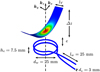Fig. 4 Geometry of the inductor and the beam (with eddy currents displayed).

4.1 Resistance measurements

4.2 Plane beam

At first, the plane beam case is considered. Figure 5 displays the resistance corresponding to the induced currents as a function of the airgap e (i.e. the vertical distance between the plane beam and the top plane of the inductor). The resistance injected in the beam is measured with a rlc-meter (plain lines with crosses). The measure is carried out at the inductor terminals, and the impedance is zeroed without the beam, to measure effectively the resistance injected in the beam. It is compared to the one computed with equation (20) (dashed lines).

The model accuracy is quite good for a width between 12 and 40 mm.

Fig. 5 Computed versus measured resistance (corresponding to the induced currents) of a plane beam (Δz = 0) as a function of the airgap e for two different beam widths (lY = 12 and 20 mm).

4.3 Elastica beam

Then, the elastica beam is considered (Fig. 6): the parameter k is changed into Δz, the height of the beam (the plane beam k → − 1 corresponding to Δz = 0). A system to get and maintain the right shape as in Figure 2, but at both ends has been elaborated. The measurement of the resistance corresponding to the power injected in the beam is carried out in the same way as for the plane beam. The noticed uncertainty is about ±1mΩ. Then, to get a valuable comparison between experiment and measurement, only the 40-mm-wide beam is considered, with various airgaps e (in the range of 1.5 − 5 mm). There is a good accordance between both, even when Δz is large.

The decentring of the elastica beam y_c, with respect to the y-axis (i.e. perpendicular to the length of the beam) is investigated (Fig. 7) at 200 kHz for various airgaps. Due to the uncertainty measurement, the 40-mm-wide beam, as in Figure 6, is considered for a medium value of Δz (11 mm). The measurements have been carried out for three positions: cantered, half-coil radius decentring, and coil-radius decentring. Computed and measured resistances are very similar. The decentring of the elastica beam x_c, with respect to the x-axis is also studied (Fig. 8). The x_c decentring is less sensitive, as the inductor remains under the beam.

The resistance of 40-mm-wide elastica beam (Δz = 11 mm) is computed as a function of the airgap e for various frequencies. The measured values are slightly above the computed ones for frequencies above 200 kHz, which can be explained by both the uncertainty measurements and the fact that H/δ increases.

Fig. 6 Computed versus measured resistance of an elastica beam (of width lY = 40 mm) as a function of the beam height Δz for different airgaps e.

Fig. 7 Computed versus measured resistance of an elastica beam (lY = 40 mm, Δz = 11 mm) as a function of the beam decentring yc.

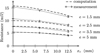Fig. 8 Computed versus measured resistance of an elastica beam (lY = 40 mm, Δz = 11 mm) as a function of the beam decentring xc.

Fig. 9 Computed versus measured resistance of an elastica beam (lY = 40 mm, Δz = 11 mm) as a function of the airgap e for different frequencies.

4.4 Full deflection model

The beam of width l_Y = 12 mm is heated by the two-wire inductor (Fig. 4). The leads are perpendicular to the beam, so they do not heat the beam. The current and the frequency are kept constant (30 A, 200 kHz). The temperature distribution is computed with equation (8) as a function of the time (Fig. 10). The initial shape of the beam (t = 0) is the one on top left of Figure 10. This shape remains the same until the temperature reaches the transformation temperature (50 °C here). The simulation shows that this temperature is reached at 0.9 s: it is consistent with the experimental beam deformation, which happens at 1 s (under the same conditions). The shape change is done with the physical support of the elastica from the original shape to the final shape (top-down left column, then top-down right one). The temperature is maximum at the centre, where the inductor is located. Since the diffusion time is high with respect to the length of the beam, the ends of the beam are not heated. After 2 s, the maximum temperature is about 75 °C.

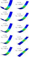Fig. 10 Temperature distribution as a function of time. θm is the maximum temperature of the beam.

5 Conclusion

A T − Ω model adapted to thin shells with the help of a change of coordinates has been introduced and confronted with experiment. The elastica, which is used as physical support allows to find the eddy current and temperature distribution as a function of time. It can be used to build a more elaborate mechanical model to take into account the large deformation.

References

All Figures

	Fig. 1 Ni-Ti Beam functioning. Top panel: time start for induction heating, middle panel: beyond the transformation temperature, bottom panel: end of the heating.
In the text

	Fig. 2 Cantilever beam for two different forces Fn.
In the text

	Fig. 3 Computation flow chart.
In the text

	Fig. 4 Geometry of the inductor and the beam (with eddy currents displayed).
In the text

	Fig. 5 Computed versus measured resistance (corresponding to the induced currents) of a plane beam (Δz = 0) as a function of the airgap e for two different beam widths (lY = 12 and 20 mm).
In the text

	Fig. 6 Computed versus measured resistance of an elastica beam (of width lY = 40 mm) as a function of the beam height Δz for different airgaps e.
In the text

	Fig. 7 Computed versus measured resistance of an elastica beam (lY = 40 mm, Δz = 11 mm) as a function of the beam decentring yc.
In the text

	Fig. 8 Computed versus measured resistance of an elastica beam (lY = 40 mm, Δz = 11 mm) as a function of the beam decentring xc.
In the text

	Fig. 9 Computed versus measured resistance of an elastica beam (lY = 40 mm, Δz = 11 mm) as a function of the airgap e for different frequencies.
In the text

	Fig. 10 Temperature distribution as a function of time. θm is the maximum temperature of the beam.
In the text

References

- T.W. Duerig, K.N. Melton, D. Stöckel, C.M. Wayman, Engineering Aspects of Shape Memory Alloys (Butterworth-Heinemann, Oxford, UK, 1990), 499 p [Google Scholar]
- S.Y. Yang, S.W. Kang, Y.M. Lim, Y.J. Lee, J.I. Kim, T.H. Nam, J. Alloys Compd. 490, L28–L32 (2010) [Google Scholar]
- R. Saunders, J. Boyd, D. Hartl, J. Brown, F. Calkins, D. Lagoudas, Smart Mater. Struct. 25, 045022 (2016) [Google Scholar]
- V.A. Jairazbhoy, P. Petukhov, J. Qu, Int. J. Solids Struct 45, 3203–3218 (2008) [Google Scholar]
- S.P. Timoshenko, J.M. Gere, Theory of Elastic Stability (Dover, New York, 2009), 560 p [Google Scholar]
Cite this article as: S. Dufour, G. Vinsard, Induction heating of a shape memory alloy beam, Eur. Phys. J. Appl. Phys. 83, 30905 (2018)