| Issue |
Eur. Phys. J. Appl. Phys.
Volume 97, 2022
|
|
|---|---|---|
| Article Number | 87 | |
| Number of page(s) | 10 | |
| Section | Plasma, Discharges and Processes | |
| DOI | https://doi.org/10.1051/epjap/2022220263 | |
| Published online | 16 December 2022 | |
https://doi.org/10.1051/epjap/2022220263
Regular Article
Interpretation of Stark broadening measurements on a spatially integrated plasma spectral line★
LAPLACE, Université de Toulouse, UMR 5213 CNRS, INPT, UPS, Toulouse, France
* e-mail: This email address is being protected from spambots. You need JavaScript enabled to view it.
Received:
18
October
2022
Accepted:
22
November
2022
Published online: 16 December 2022
Abstract
In thermal plasma spectroscopy, Stark broadening measurement of hydrogen spectral lines is considered to be a good and reliable measurement for electron density. Unlike intensity based measurements, Stark broadening measurements can pose a problem of interpretation when the light collected is the result of a spatial integration. Indeed, when assuming no self-absorption of the emission lines, intensities simply add up but broadenings do not. In order to better understand the results of Stark broadening measurements on our thermal plasma which has an unneglectable thickness, a Python code has been developed based on local thermodynamic equilibrium (LTE) assumption and calculated plasma composition and properties. This code generates a simulated pseudo experimental (PE) Hα spectral line resulting from an integration over the plasma thickness in a selected direction for a given temperature profile. The electron density was obtained using the Stark broadening of the PE spectral line for different temperature profiles. It resulted that this measurement is governed by the maximum electron density profile up until the temperature maximum exceeds that of the maximum electron density. The electron density obtained by broadening measurement is 60–75% of the maximum electron density.
The present article is published after the retraction of the paper https://doi.org/10.1051/epjap/2022220008 after the authors detected an error in the numerical determination of the PE spectral line. All errors have been corrected. The corrections in respect to the retracted paper can be found highlighted in yellow in the Supplementary material at: https://www.epjap.org/10.1051/epjap/2022220263/olm.
© J. Thouin et al., Published by EDP Sciences, 2022
 This is an Open Access article distributed under the terms of the Creative Commons Attribution License (https://creativecommons.org/licenses/by/4.0), which permits unrestricted use, distribution, and reproduction in any medium, provided the original work is properly cited.
1 Introduction
For the experimental characterisation of an electric arc, emission spectroscopy is the diagnostic method of choice for the measurement of the plasma temperature or species densities. Among the different spectroscopic diagnostic methods, those based on the measurement of the Stark broadening of a spectral line are widely used [1–6].
In order to perform a spatially resolved spectroscopic measurement within the plasma there are several methods. When an assumption of plasma axisymmetry can be made, methods based on Abel inversion can be used [6,7]. When this assumption is no longer valid and the optical system allows simultaneous acquisitions in different directions, tomographic reconstruction methods can be considered [8].
However, when none of these methods can be applied, because the plasma is not axisymmetric, the time constraints are too great, the intensity of the discharge is not sufficient to allow the selection of light rays or because the experimental setup does not allow a complex optical setup, it is common to collect the light emitted by the plasma using a focusing optical setup or selecting a direction with pinholes [1,3,5,9]. In this case the light is collected over the entire thickness of the plasma and the broadening measurement is made on the spectral line resulting from the integration over the thickness of the plasma. For inhomogeneous plasma and depending on the measurement performed, it can be complex if even possible to interpret the measured quantity.
The presented study was performed in order to interpret experimental results of Stark broadening measurements on H α spectral line emitted by a water thermal plasma. This plasma, considered at local thermodynamic equilibrium (LTE), is generated by a ten milliseconds electric arc in a water tank which vaporizes the water. The light is collected in a direction selected using a couple of pinholes. We are interested in the theoretical determination of the electron density by measurement of the broadening of a spectral line. We are interested in the hydrogen spectral line Hα for which we consider the Stark effect as the dominant source of broadening in the presence of a high electron density [2].
In order to study the relevance of the broadening measurement to obtain the electron density, we will first define the context of our study. Then, we will present the parameters that govern the profile of a spectral line: (1) the emissivity of the transition associated with the Hα spectral line which will be calculated from the plasma composition and (2) the Stark broadening of the Hα line determined by simulation from the work of Gigosos et al. [10] We will then perform a parametric study using different temperature profiles for the water thermal plasma. We will focus on the electron density determined from the reconstructed Hα pseudo experimental (PE) spectral line for these different profiles assuming that the broadening is only due to Stark effect. Finally, we will conclude on the meaning of the obtained measurements.
2 Context of this study
We performed experimental emission spectroscopy measurements on a water plasma. This plasma was generated between two vertical sharpened rods of tungsten (see Fig. 1). In order to generate the arc, a half sine wave of current is applied through a fuse wire. The wire is vaporized by Joule effect and generates a water vapour bubble which gradually expands before collapsing. The duration of the discharge is 10 ms and the sinusoidal current wave (f = 50 Hz) has an amplitude of about 1 kA. A theoretical study of the phenomenon was carried out in our team [11] in order to understand the behaviour of the plasma. A water plasma bubble was simulated using the commercial software @fluent based on the finite volume method. Plasma properties have been calculated for water, the theory is presented in Harry-Solo et al. [12]. First instants of the bubble formation are not described; the simulation begins with a conducting channel already established. Using the experimental variations of the measured voltage and current intensity, a source term is applied within a volume defined by a boundary temperature of 7 kK. This arbitrary temperature defines the conducting channel. Naturally, this volume changes during the deposition of energy. The phase transition between vapour and liquid was handled using a model based on that of Lees [13]. This study gave us a homogenous value for the pressure inside the vapour bubble close to 3 bar at very early times of the expansion (t < 0.5 ms). Therefore, in this article the plasma will be considered to be pure water and its properties calculated for a pressure of 3 bar.
To illustrate, Figure 1 shows the observed bubble with the plasma contained in the saturated zone. This image was obtained using a Photron FASTCAM SA5 high-speed camera, the exposure time was 1/25,000 s and three neutral density filters were fitted on the lens with an attenuation factor respectively of 64, 32 and 16. The acquisition method is described with more details in [14]. The circle in the foreground corresponds to the shape of the observation window. A halogen lamp is used as backlighting, its filament is visible horizontally in the background. Backlighting is only necessary to improve the observation of the edge of the water vapour bubble. Two copper electrode holders support the tungsten rods of 1.6 mm diameter vertically. Between the two electrodes is placed a 0.13 mm copper wire.
The light emitted by the plasma is collected through two irises which select a beam of light. When considering no self-absorption, the light collected is the sum of all emissions on the line of sight selected by the two pinholes, see Figure 2.
Figure 2 shows the light being collected on the line of sight I(X0). We can consider that the profile of one emission spectral line, at a given wavelength, integrated over this string of plasma is the sum of the local emissions at that same wavelength along the string. These local emission spectral lines can be characterized using the local conditions of emission. We will describe this process in Section 4.
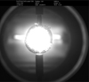 |
Fig. 1 Image of a water vapour bubble. The image is saturated in the centre by the emission of light from the arc. |
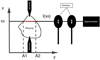 |
Fig. 2 Plasma light selection and acquisition. |
3 Spectral emission line description
The shape of a spectral line profile can be characterized using different parameters such as its amplitude or its broadening. The area covered by the profile of the spectral line is dependent on those two previous parameters but also on the shape of the profile. These different parameters are illustrated in Figure 3. The full width half area FWHA of the spectral line is the width of the hatched area. The full width at half maximum FWHM is plotted as well.
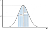 |
Fig. 3 Intensity of a given spectral line plotted against the wavelength; Illustration of FWHM and FWHA parameters. |
3.1 Broadening
The physical causes of spectral line broadening in a thermal plasma are numerous, however, a natural broadening (small) as well as a broadening due to the optical system and finite resolution of the spectrometer, are always present. In addition, depending on the plasma and spectral emission line considered, Doppler, Van der Walls or Stark broadenings can be present. Depending on its cause, the broadening profile will be either Gaussian (for the optical and Doppler broadenings) or Lorentzian (for the natural broadening and collisional broadenings such as Van der Walls or Stark). The different causes of broadening of a spectral line are discussed in detail in the work of Griem [15]. The resulting spectral line profile is a Voigt profile, i.e. a convolution of a Lorentzian and a Gaussian profile. It can lean towards a Gaussian or a Lorentzian profile depending on the sources of broadening. If several sources of broadening are present, some of them depending on the emission environment and therefore the position of emission, reconstructing the profile of the integrated line can be difficult.
In this work, we are interested in the Hα spectral line for which the Stark broadening is such that all other sources of broadening are negligible [2]. The resulting profiles tend to be Lorentzian.
The broadening of Hα is provided to us directly as a function of the electron density ne(x,y,z) by the equation determined by Gigosos et al. [10] with the FWHA:
 (1)
(1)
A Lorentzian is defined as:
 (2)
(2)
with: –λ = wavelength. –A = amplitude factor. –2σ = FWHM; n e = electronic density.
The indefinite integral is:
 (3)
(3)
And the area a l of the profile is:
 (4)
(4)
Let's assume that  gives the FWHA so that:
 (5)
(5)
 (6)
(6)
Which is true for:  therefore
  and
and  .
.
It should be noted that the FWHA is equal to 2σ, which is also the FHWM for a Lorentzian profile.
3.2 Emissivity
In order to reconstruct the integrated spectral line emitted by the plasma in one direction, the amplitude of the spectral line or its intensity (area) is necessary in addition to the broadening profile. This information is provided by the emissivity of the spectral line. The emissivity associated with an electronic transition from an energy level i to an energy level j is expressed as:
 (7)
(7)
with:
J (λ) emissivity profile as a function of the wavelength.
ni population density of the emitting level i.
Aij Einstein coefficient for the electronic transition from level i to j.
P, T pressure and temperature.
h, c Planck's constant and speed of light in vacuum.
If the plasma is assumed to be at local thermodynamic equilibrium (LTE) then the density ni of the level i is given by Boltzmann law:
 (8)
(8)
with:
n (P, T) global species density:
 with k being the excitation level.
Z (P, T) partition function for the considered species.
Ei energy for the level i.
gi degeneracy of the level i.
K : Boltzmann constant.
The emissivity can be expressed as:
 (9)
(9)
And λt is the wavelength of the light emitted by the electronic transition considered.
To summarize, for a Lorentzian profile we have:
The area al ∝ Jtot and it is equal to: al = Aσ.
FWHM = FWHA = 2σ.
 .
.
The evolution of the emissivity of the Hα spectral line as a function of pressure and temperature, the parameters gi,Aij and the other constants do not vary if we consider a single electronic transition. In equation (9) Jtot depends on pressure and temperature via the terms n (P, T) , Z (P, T), and  . For the electronic transition associated with Hα, Ei is equal to 12.0875 eV [16].
For a thermal plasma considered to be in LTE, solving the corresponding equations (Saha-Eggert, Guldberg-Waage, electrical neutrality, Dalton law) gives us the evolution of the plasma species densities as a function of pressure and temperature. The method is detailed in Harry-Solo et al. [12]. Thus, the species global densities and their partition function are known as a function of pressure and temperature. In our study, the composition of a pure water plasma is calculated for a pressure of 3 bar according to previous study by Laforest [11]. Using these data and the equation (9) we can determine the evolution of the emissivity of the Hα line as a function of temperature (see Fig. 4).
Figure 4 shows that the maximum emissivity is reached around 17 kK. As indicated by equation (9) this evolution results from the combination of different parameters. This maximum occurs at higher temperatures than the maximum density of the emissive species, hydrogen. This is explained by the contribution of the terms Z (P, T) and  in equation (9) which compensate for the decrease in hydrogen density. The evolution of the emissivity was calculated using only the temperature and pressure dependent terms. The other terms are dependent on the electronic transition and have therefore been ignored as we are studying the evolution of a single transition. This is the reason why we have represented the normalised emissivity in Figure 4. It can also be noted on Figure 4 that the maximum electron density occurs at a higher temperature(≈ 19.4 kK) than the maximum emissivity of the Hα line (≈ 17 kK) .
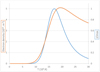 |
Fig. 4 Evolution of the normalised emissivity of the Hα line (blue) and the electron density (orange) as a function of temperature for a water plasma at 3 bar. |
4 Results
4.1 Different temperature profiles
We consider an axisymmetric plasma of constant pressure (3 bar) to study the profile of the Hα pseudo experimental (PE) spectral line reconstructed from different temperature profiles. The composition of a pure water plasma calculated from our model [12] provides the electron density profile corresponding to the temperature profile. The objective is to study the electron density deduced from measurement of the Stark broadening of this reconstructed PE line with equation (1) provided by Gigosos et al. [16]. This electron density will be compared with the electron density profile.
We arbitrarily defined four axisymmetric temperature profiles and two asymmetric ones, with a maximum temperature in the centre. These temperature profiles are common and could correspond to any type of axisymmetric plasma with the light collected in a direction perpendicular to the symmetry axis. The maximum temperature (≈16 kK) was initially chosen to be lower than that of the maximum emissivity of the Hα line (≈17 kK). These different temperature profiles are given in Figure 5 (left) with the corresponding electron density profiles (right).
From these profiles and the elements determined in Section 4, six Hα PE spectral lines are calculated as the sum of Lorentzian spectral lines on a plasma string whose temperature follows one of the temperature profile. The reconstruction of this spectral line was performed numerically using an in-house developed Python program. A sum of Lorentzian profiles calculated on each point of the temperature profile is performed:
 (10)
(10)
Using:


Although the sum of Lorentzian profiles with different amplitudes and broadenings does not lead to a simple analytical expression of a Lorentzian, it is possible to treat this PE spectral line the same way we would an experimental one. It is common to fit integrated experimental spectral lines with the best matching Voigt or Lorentzian profile. The Lorentzian profile that best matches that of the PE spectral line is calculated using the lmfit library in Python and the broadening of this Lorentzian profile is measured.
The PE spectral line determined this way and the associated Lorentzian profile are plotted in Figure 6 for temperature profile number 4 (P4). Figure 6 shows that a Lorentzian profile allows most points to be approached correctly, with the exception of those close to the maximum. The error on the estimation of the maximum is calculated and tabulated for the different profiles. As indicated in the table of Figure 6, the discrepancy between the data and the fit is most pronounced for profile number 4. The profile number 4 (P4) is also the least realistic profile.
We will detail the case of the fourth temperature profile (Fig. 5, P4) which shows the largest deviation. We have numerically determined the FWHA of the line determined by the calculation and compared it to that of the Lorentzian profile:
 (11)
(11)
We have calculated the deviation on the electron density measurement presented in the same way:
 (12)
(12)
This deviation is not negligible, but it has been determined for the profile with the largest deviation between the data and the fit (P4). Experimentally, we usually perform the broadening measurement (FWHA or FWHM) on the fit, and when several sources of broadening are mixed, a Voigt profile is sometimes considered with the assumption that the Lorentzian component is solely due to Stark effect. For the different lines determined, a Voigt profile does not allow a better fit of the line. However, the difference between the FWHA measurement made directly on the PE spectral line data and the fit is too large to be ignored. This is why in this study we will perform our broadening measurements on the PE spectral line data without using any fit.
The electron density profiles are calculated with equation (1) from the broadening measurements and presented in Figure 7 (hatched in black is the mean electron density over the profile and hatched in white is the density resulting from the broadening measurement).
We observe in Figure 7 that the mean electron density for the first profile is 0.49 × 10²³ m−3 and the maximum is 4.05 × 10²³ m−3. The density value determined from the line broadening is 2.49 × 10²³ m−3. This value is closer to the maximum than it is to the mean value of the profile. For all profiles, the density determined seems to be driven in greater part by the hottest and most electronically dense area (which will also be the most emissive area) than by the other parts of the profile. On profile P3, the electron density determined by the measurement is closest to the maximum; it is also for this profile that the warmest zone in the centre is the largest. For the temperature profile P5, which is a combination of profiles P3 and P4, the broadening measurement seems to be driven by profile P3 and less affected by the thinner (especially in the warm central zone) profile P4 which results in an electron density measurement rather close to the maximum. Profiles P1 and P2 are both Gaussian and are temperature profiles with a similar maximum temperature (and therefore with a similar maximum value of the electron density), differences exist in the peripheral zones of the plasma where profile P2 presents a higher electron densities as it is defined by a wider Gaussian profile. On the profiles P1 and P2 the densities obtained by broadening measurements are almost identical and represent the same fraction of their respective electron density profile maxima, although the average electron density is higher for profile P2. It is also true for profile P6, unsurprisingly, given that it is a combination of profiles P1 and P2. Excluding the highly unrealistic fourth profile P4, all electron densities obtained by broadening measurement represent a similar fraction of their respective electron density profile maxima, i.e. between 62% and 73%.
It should be noted that the maximum temperature of these profiles (≈16 kK) is lower than the maximum emissivity temperature for the Hα spectral line (≈17kK) as well as the temperature of the maximum electron density (≈19.4 kK). In Section 5.2 we will study the influence of the maximum temperature, especially when it exceeds these two maxima.
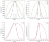 |
Fig. 5 Temperature profiles 1 and 2 are Gaussian, profile 3 is arbitrary and profile 4 is linear. Temperature profiles 5 and 6 are asymmetric and are respectively half of profiles 3 and 4 and half of profiles 1 and 2. The electron density profiles are deduced from the plasma composition. |
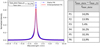 |
Fig. 6 Comparison between the spectral line determined for the temperature profile 4 and its Lorentzian fitted profile (Left side). Table of the error in percentage on the estimation of the maximum for each profile (Right side). |
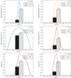 |
Fig. 7 Electron density profiles, average over the profile and electron density measured by broadening measurement. |
4.2 Different values of the maximum temperature
We defined four Gaussian temperature profiles with the same width at half height but with different amplitudes. The four temperature profiles (P1–P4) and the associated electron density profiles (N1–N4) are shown in Figure 8.
Figure 8 shows that the maximum temperature of the first two profiles is chosen lower than the maximum emissivity temperature of the Hα spectral line. Profile P3 has a maximum temperature very slightly above the maximum electron density, while profile P4 has a much higher maximum temperature. We also observe in Figure 8 a dip in electron density in the centre with profile N3 which is even more pronounced on profile N4. This dip is a consequence of the temperature in the centre exceeding that of the maximum electron density. In the same way as in Section 4.1, the measured electron density is determined from the broadening of the Hα spectral line calculated from these temperature profiles. These results are presented in Figure 9 with the electron density profiles (hatched in black is the mean electron density over the profile and hatched in white is the density resulting from the broadening measurement).
The measured electron density (Fig. 9) increases up to and including profile 3 (N3). Thus the maximum emissivity of the Hα spectral line does not seem to limit the measurement; it is still possible to measure electron densities corresponding to higher temperatures. Conversely, we do not observe an increase in electron density determined by broadening measurement on profile P4/N4 compared to that of profile P3/N3 even though the average electron density on the profile has increased. As soon as the temperature of the maximum electron density is exceeded, the electron density measured stops increasing (for a Gaussian profile maintaining the same width at half-height) which seems to indicate a similar temperature when in fact it has increased. If we consider Figure 4, we could also assume that we have exceeded the temperature of the maximum electron density (which is the case) and interpolate with higher temperatures. In this case, the temperature is overestimated. For example, we would measure more than 30 kK for profile P4. Despite this, just as in Section 4.1, for all four profiles the electron density determined by broadening is somewhere between 61% and 70% of the maximum of the profile.
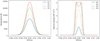 |
Fig. 8 Gaussian temperature profiles presenting identical width at half height but different maxima. The electron density profiles are deduced from the temperature profiles. |
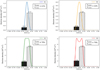 |
Fig. 9 Electron density profiles, mean value over the profile and density obtained by broadening measurement. |
5 Conclusion
The electron density measured from the broadening of the Hα PE spectral line determined as a sum over a temperature profile was studied. The study was conducted for temperature profiles with different shapes and maxima. It seems that the electron density obtained this way is governed by the maximum of the electron density profile and that it is only marginally affected by the rest of the electron density profile. The measurement is therefore rather uncorrelated with the average electron density. It was also observed that exceeding the maximum emissivity temperature of the spectral line considered did not present any particular problem. In our study, the problem lies with profiles whose temperature is such that it exceeds that of the maximum electron density at the core of the profile and induces a density dip. For these profiles, the broadening measurement is hardly usable.
It is interesting to note that the electron densities determined by broadening of the PE spectral lines represent, for all but one unrealistic profile (P4), a similar fraction of their respective electron density profiles maxima. This result is true for temperature profiles of different shapes, as shown in Section 4.1, and for Gaussian temperature profiles with the same width at half height but with different maxima, as shown in Section 4.2. The electron density measured by broadening measurement is 60–75% of the maximum electron density.
Author contribution statement
JT developed the computer code, carried out the analysis of the results and wrote the manuscript. MB contributed to the drafting of the project, PF and JJG reviewed the manuscript and provided data for the analysis. PF conceptualised the problem.
Supplementary material
References
- P. Vanraes, A. Nikiforov, C. Leys, Electrical and spectroscopic characterization of underwater plasma discharge inside rising gas bubbles, J. Phys. Appl. Phys. 45, 245206 (2012) [CrossRef] [Google Scholar]
- R. Venger, T. Tmenova, F. Valensi et al., Detailed investigation of the electric discharge plasma between copper electrodes immersed into water, Atoms 5, 40 (2017) [CrossRef] [Google Scholar]
- V.S. Burakov, E.A. Nevar, M.I. Nedel'ko et al., Spectroscopic diagnostics for an electrical discharge plasma in a liquid, J. Appl. Spectrosc. 76, 856 (2009) [CrossRef] [Google Scholar]
- F. Wang, Y. Cressault, P. Teulet et al., Spectroscopic investigation of partial LTE assumption and plasma temperature field in pulsed MAG arcs, J. Phys. D:Appl. Phys. 51, 255203 (2018) [Google Scholar]
- T. Namihira, S. Sakai, T. Yamaguchi et al., Electron temperature and electron density of underwater pulsed discharge plasma produced by solid-state pulsed-power generator, IEEE Trans. Plasma Sci. 35, 614 (2007) [CrossRef] [Google Scholar]
- G. Ni, P. Zhao, C. Cheng et al., Characterization of a steam plasma jet at atmospheric pressure, Plasma Sources Sci. Technol. 21, 015009 (2012) [CrossRef] [Google Scholar]
- A. Mašláni, V. Sember, M. Hrabovský, Spectroscopic determination of temperatures in plasmas generated by arc torches, Spectrochim. Acta B 133, 14 (2017) [CrossRef] [Google Scholar]
- J. Benech, Spécificité de la mise en oeuvre de la tomographie dans le domaine de l'arc électrique: validité en imagerie médicale. These de doctorat, Toulouse 3 (2008) [Google Scholar]
- H. Pauna, M. Aula, J. Seehausen et al., Optical emission spectroscopy as an online analysis method in industrial electric arc furnaces, Steel Res. Int. 91, 2000051 (2020) [CrossRef] [Google Scholar]
- M. Gigosos, M. González, V. Cardeñoso-Payo, Computer simulated Balmer-alpha, −beta and −gamma Stark line profiles for non-equilibrium plasmas diagnostics, Spectrochim. Acta B 58, 1489 (2003) [CrossRef] [Google Scholar]
- Z. Laforest, Etude expérimentale et numérique d'un arc électrique dans un liquide. These de doctorat, Toulouse 3 (2017) [Google Scholar]
- A. Harry Solo, M. Benmouffok, P. Freton, J.-J. Gonzalez, Stochiometry air − CH4 mixture: composition, thermodynamic properties and transport coefficients, Plasma Phys. Technol. 7, 21 (2020) [CrossRef] [Google Scholar]
- W.H. Lee, A pressure iteration scheme for two-phase flow modelling, in Computational Methods for Two-Phase Flow and Particle Transport (World Scientific, 2013), pp. 61–82 [CrossRef] [Google Scholar]
- Z. Laforest, J.J. Gonzalez, P. Freton, Experimental study of a plasma bubble created by a wire explosion in water, IJRRAS 34, 93 (2018) [Google Scholar]
- H. Griem, Spectral Line Broadening by Plasmas (Elsevier Science, Oxford, 1974) [Google Scholar]
- A.E. Kramida, A critical compilation of experimental data on spectral lines and energy levels of hydrogen, deuterium, and tritium, At. Data Nucl. Data Tables 96, 586 (2010) [CrossRef] [Google Scholar]
Cite this article as: Julien Thouin, Malyk Benmouffok, Pierre Freton, Jean-Jacques Gonzalez, Interpretation of Stark broadening measurements on a spatially integrated plasma spectral line, Eur. Phys. J. Appl. Phys. 97, 87 (2022)
All Figures
|
Fig. 1 Image of a water vapour bubble. The image is saturated in the centre by the emission of light from the arc. |
| In the text | |
|
Fig. 2 Plasma light selection and acquisition. |
| In the text | |
|
Fig. 3 Intensity of a given spectral line plotted against the wavelength; Illustration of FWHM and FWHA parameters. |
| In the text | |
|
Fig. 4 Evolution of the normalised emissivity of the Hα line (blue) and the electron density (orange) as a function of temperature for a water plasma at 3 bar. |
| In the text | |
|
Fig. 5 Temperature profiles 1 and 2 are Gaussian, profile 3 is arbitrary and profile 4 is linear. Temperature profiles 5 and 6 are asymmetric and are respectively half of profiles 3 and 4 and half of profiles 1 and 2. The electron density profiles are deduced from the plasma composition. |
| In the text | |
|
Fig. 6 Comparison between the spectral line determined for the temperature profile 4 and its Lorentzian fitted profile (Left side). Table of the error in percentage on the estimation of the maximum for each profile (Right side). |
| In the text | |
|
Fig. 7 Electron density profiles, average over the profile and electron density measured by broadening measurement. |
| In the text | |
|
Fig. 8 Gaussian temperature profiles presenting identical width at half height but different maxima. The electron density profiles are deduced from the temperature profiles. |
| In the text | |
|
Fig. 9 Electron density profiles, mean value over the profile and density obtained by broadening measurement. |
| In the text | |
Current usage metrics show cumulative count of Article Views (full-text article views including HTML views, PDF and ePub downloads, according to the available data) and Abstracts Views on Vision4Press platform.
Data correspond to usage on the plateform after 2015. The current usage metrics is available 48-96 hours after online publication and is updated daily on week days.
Initial download of the metrics may take a while.