| Issue |
Eur. Phys. J. Appl. Phys.
Volume 97, 2022
|
|
|---|---|---|
| Article Number | 13 | |
| Number of page(s) | 5 | |
| Section | Imaging, Microscopy and Spectroscopy | |
| DOI | https://doi.org/10.1051/epjap/2022210260 | |
| Published online | 01 March 2022 | |
https://doi.org/10.1051/epjap/2022210260
Regular Article
Bright sources under the projection microscope: using an insulating crystal on a conductor as electron source
CINaM, Aix-Marseille Univ, CNRS, UMR 7325,
13288
Marseille, France
* e-mail: This email address is being protected from spambots. You need JavaScript enabled to view it.
Received:
17
November
2021
Received in final form:
7
January
2022
Accepted:
24
January
2022
Published online: 1 March 2022
Abstract
The development of bright sources is allowing technological breakthroughs, especially in the field of microscopy. This requires a very advanced control and understanding of the emission mechanisms. For bright electron sources, a projection microscope with a field emission tip provides an interference image that corresponds to a holographic recording. Image reconstruction can be performed digitally to form a “real” image of the object. However, interference images can only be obtained with a bright source that is small: often, an ultra-thin tip of tungsten whose radius of curvature is of the order of 10nm. The contrast and ultimate resolution of this image-projecting microscope depend only on the size of the apparent source. Thus, a projection microscope can be used to characterize source brightness: for example, analyzing the interference contrast enables the size of the source to be estimated. Ultra-thin W tips are not the only way to obtain bright sources: field emission can also be achieved by applying voltages leading to a weak macroscopic electric field (< 1V∕μm) to insulating micron crystals deposited on conductors with a large radius of curvature (> 10 μm). Moreover, analyzing the holograms reveals the source size, and the brightness of these new emitters equals that of traditional field emission sources.
© L. Lapena et al., published by EDP Sciences, 2022
 This is an Open Access article distributed under the terms of the Creative Commons Attribution License (https://creativecommons.org/licenses/by/4.0), which permits unrestricted use, distribution, and reproduction in any medium, provided the original work is properly cited.
1 Introduction
Using a bright source is essential in microscopy applications. Moreover, the wave-like nature of particles is best observed using a bright source. It is only after the invention of the laser that the holography described and demonstrated by Gabor [1] was really implemented. Brightness corresponds to the emitted intensity at a given energy I(E) under an angle of cone Ω coming from a zone s on the source itself:  . For a given intensity, the smaller the source, the brighter it is and the more spatially coherent the beam. A thermo-electronic electron source such as a heated filament, although very intense, cannot match the brightness of field emission sources such as an ultra-thin tungsten tip: the emission area is much too large. The tips may end with only a few atoms. All the intensity comes from an extremely small area. The brightness is three orders of magnitude higher than a filament source [2]. A more recent example is the Helium ion source used in the Helium microscope. Economou et al. [3] explain the various obstacles that had to be overcome before using these sources in an ion column to reach resolutions of 0.35 nm on the sample. The contrasts obtained in this microscope are unequaled. It took 20 years to go from the tungsten trimer to the reliable and reproducible beam. The first studies on these emitters were carried out with a field ion microscope. This article reveals that a projection microscope is perfectly suited to characterizing sources [4,5], explaining how it can be used to determine source size, whatever the emitted particles. Two sources are used: a coaxial ion source integrating an ultra-thin tungsten tip and an electron source composed of an insulating crystal deposited on a carbon fiber. While this electron source has already been described in several articles [6,7], we recall here the different experimental setups allowing its use in a projection microscope.
2 Source-size measurement in a projection microscope
The projection microscope is a derivative of the field-ion or field-electron microscope, where only the emission profile and the structure of the emitter itself are observed. Instead of using a diaphragm as an extractor, the projection microscope uses an “open object” such as a lacey or holey carbon film deposited on a copper grid. The image of the object is then projected onto a screen. Being open, the lacey or holey carbon grids let the beam pass through them directly; their dimensions also vary, and they can be as small as a few nm [8]. In order to position the object precisely in front of the source, it is placed on a piezoelectric manipulator. The detector usually consists of one or more micro-channel plates (MCP) and a fluorescent screen. The amplification depends on the number of MCP and the voltage applied to the MCP stack. The resolution of the detector in analog mode is about 100 μm, but in particle-counting mode it is reduced to the plate pitch, i.e. about 15 μm [9]. The image obtained with this type of microscope depends on the nature of the particles emitted, even at equivalent magnifications. The magnification factor is the ratio of the source-to-screen distance, D, to the source-to-object distance, d:  . The object is first positioned far from the source. From the grid pitch, the magnification can be determined precisely. Then, the object is moved closer and magnification gradually increases. Depending on the particle and the dimensions, fringes can be observed. In the case of a point source facing a point object, the position of the constructive fringes with respect to the center of the interference pattern is calculated as follows:
  with
with  the wavelength associated with the particle of mass m and energy E (h is the Planck constant) and p the interference order. For an electron emitted at 100V, the wavelength is 1.2 Å. If the object is 100μm from the source, in a 1m projection microscope, the first fringe is 1.55 mm from the center and then the fringes get closer and closer. For ions, even when very light, such as hydrogen ions of 1 keV, the wavelength is then 0.9 pm and the first fringe is 134 μm from the center. In a projection set-up with metric dimensions, no fringe will be seen in analog detection mode. Observations of fringes depends on the square root of the wavelength ratio
  : if the wavelength is 100 times smaller, the projection distance must be 10 times greater to observe the same effect. Source size is characterized via the projection microscope according to the contrast on the image, but the treatment is particle-dependent.
In the case of ion sources, because no fringes are observed in our set-up, the contrast can be measured directly. As in the case of Leonardo da Vinci’s camera obscura, the spatial resolution can be obtained on the edge of an object by an error function [10]. In this way, the smallest observable detail is measured and corresponds to the maximum size of the source used to produce that image. In Figure 1, the size of the coaxial ion source, presented in various articles [11,12] is measured. Different species are first separated with a magnetic field (H+, H2+, and H3+). Their formation and intensity ratio depend on the tip shape and on the electric field strength [13,14]. They are then analyzed separately: the size of each ion source is about s = 2.2 nm.
In the case of electron sources, the contrast cannot be measured directly because fringes are observed. To measure the source size for electrons, two methods are used: the last visible fringe [6], and the contrast in an interferometry experiment [15].
-
The last visible fringe (at
 ) corresponding to the smallest visible detail is measured; the source is smaller than:
  . To determine source size s < 10 nm, the image needs to be sufficiently magnified: in a D = 1 m projection microscope, the source-object distance has to be smaller than d < 1 μm. In the case of an ultra-thin metal tip, this is a common requirement. However, if the support of the source is too bulky, as with the so-called “celadonite source” [6], it is impossible to respect this distance without touching the extractor grid. To overcome this difficulty, an electrostatic lens can be used to enlarge the fringe recording. In the example of Figure 2, source size is estimated to be below s < 2.6 nm.
This recording corresponds to the first step of holography. A digital reconstruction procedure can be applied to find the shape of the object [16,17]. With more complex objects, where several fringe patterns merge, the reconstruction can also be used to determine the source size: the source is smaller than the smallest observable detail. Physically, this form of determination amounts to measuring the smallest visible fringe. Generally, the reconstruction with the best contrast is chosen, the source-to-object distance is determined from this reconstruction, and the source size can be estimated from the error function applied to the final image. Figure 3 shows the reconstruction of a hologram produced from the celadonite source. The reconstruction procedure used was the one presented in [16] and does not eliminate the twin-image problem as suggested in [18]. Nevertheless, it gives a source size of below s < 2 nm.
-
Measuring the contrast in an interferometry recording is the most accurate way to deduce the size of the electron source. This method applied to the emission of electrons by an ultra-thin tungsten tip made it possible to measure sWtip = 0.16 nm [15,19]. For an ultra-thin tungsten tip, brightness is measured as B = 109 A cm−2 sr−1. If a small filament is positively charged, the electron beam appears to come from 2 sources separated by a, which depends on the filament charge. Fringes are then regular (
 ), with an intensity modulation that results from the sharp cutoff in wave vector direction right after the biprism. The contrast
  depends on source size [20]:
  . This method is illustrated in Figure 4; to obtain such a contrast (Γ = 0.33 > 0.217), the size of the source needs to be within the first lobe of the sinc
curve. The sinc curve can be turned into a sum, giving:
. This method is illustrated in Figure 4; to obtain such a contrast (Γ = 0.33 > 0.217), the size of the source needs to be within the first lobe of the sinc
curve. The sinc curve can be turned into a sum, giving:  . Here, the source size is estimated at s < (1.5 ± 0.3) nm.
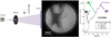 |
Fig. 1 The size of the ion source is determined by measuring the contrast at the edge of the shadow of an object. Magnification: G = 180000, ion source potential V = 2 kV, source-screen distance D = 40 cm, source-object distance d = 2.2 μm |
 |
Fig. 2 The size of a bulky electron source (so-called celadonite source) is determined by using a lens to enlarge the recording hologram and measuring the smallest detail on the image: the last visible fringe order (pl = 18). Here, the source size is s < 2.6 nm. Magnification: G = 235000, electron source potential V = −280 V, source-screen distance D = 86 cm, source-object distance d = 13.3 μm. |
 |
Fig. 3 Left side: hologram obtained in a point-projection microscope with a celadonite source and, right side: its reconstruction. The inset corresponds to the profile along a horizontal line on the reconstruction. The error function applied to the profile of the “best contrast” reconstructed image gives a source size of s < 2 nm. |
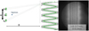 |
Fig. 4 Interferometry experiment carried out with a charged filament using the celadonite source. Electron energy: Ee = 227 eV, projection distance D = 86 cm, inter-source distance: a = 280 ± 30 nm, source-object distance d = 15 ± 3 μm, fringe-to-fringe distance i = 0.24 mm. Contrast Γ depends on source size, here estimated at s < 1.5 nm. The biprism is a charged ϕ = 118 nm diameter filament of an electrical grounded lacey carbon film. |
3 An insulating crystal-on-conductor electron source
In early versions of the electron source composed of an insulating crystal (celadonite) deposited on a carbon fiber, crystals were deposited on carbon films. This meant that several crystals would emit but the intensity plotted against the voltage indicated a Fowler-Nordheim regime followed by a saturation regime. The Fowler-Nordheim regime (ln(I∕V2) = f(1∕V) is linear [14]) means that field emission is observed. In order to characterize the beam from a single crystal, the intention was to use the point-projection microscope, so the source-object distance had to be small. Thus, insulating crystals are now deposited with a micropipette at the end of a carbon fiber, so that the object is closer to the source. The I(V) (see Fig. 5) curve remains the same, except that the voltage is lower because the shape of the conductive substrate leads to a higher electric field. The macroscopic field responsible for the emission remains the same, in the order of some V∕μm.
The crystal is perfectly flat and thin on the rough conductive surface. When the fiber is polarized, the crystal surface charges to a potential different from the fiber, creating local field enhancement. This exaltation was deduced from the instabilities measured on the emitted intensity, which can also be seen on Figure 5. When the intensity is analyzed more closely over time, current jumps related to the number of charges present on the surface of the crystal are recorded (for further information see [21]). At nanoscale, the roughness of the conductor enhances the local field. When this local field reaches some V∕nm, electron emission takes place. However, this source is not an ultra-thin tip; it is situated at the end of a carbon fiber of ϕ = 10 μm diameter, and the approach is therefore limited to some tens of micrometers [6]. For this reason, a new point-projection microscope was realized and presented in [7]. It comprises a micro-manipulator, a double electrostatic Einzel lens described in [22,23], and a double micro-channel plate detector. It was shown that the spherical aberration of the lens is smaller than the detector grain and that distortion is limited by an entrance diaphragm of 100μm diameter. For the screen, a double micro-channel plate was chosen based on the gain in resolution reported in [9] when the detector is used in counting mode. These modifications enabled us to achieve a source size of s = 1.5nm according to the interferometric measurement described above. This measurement was carried out by accumulating 200 images with a pause time of 111ms each, in counting mode. We are grateful to an anonymous referee for pointing out that the shorter this time, the better the contrast (mainly due to system vibration). But here, using the counting mode does not accelerate the procedure, which strongly suggests that the source size is much smaller than measured here. Integrating all the data available in this article (I = 30 μA, Ω = 0.8 sr and s = 1.5 nm), the brightness of the celadonite source was estimated at B = 0.5 × 10⁹ A cm−2 sr−1. A minimum source-to-object distance of the order of d = 12 μm was maintained, key if aiming at sufficiently comfortable off-axis holography.
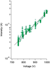 |
Fig. 5 Typical intensity versus voltage curve for a celadonite source. Intensity fluctuation at a fixed voltage reflects instabilities due to the charge of the insulating crystal [21]. |
4 Conclusion
In summary, the point-projection microscope provides contrast that is directly dependent on the size of the source. This makes it particularly useful for studying sources. It is not always possible to use the simple projection system, but the use of lenses or high-precision detectors has been shown to help increase the resolution. A new electron source composed of an insulating crystal deposited on a conductive fiber has a brightness equivalent to that of conventional field emission sources (ultra-thin metal tip). It is robust, easy to prepare, and has a long lifetime, even at high pressure. To study this source, a special point-projection microscope was developed to meet the challenge of maintaining a minimum source-to-object distance of d > 12μm. Today, this new type of microscope holds promise for a number of applications, like off-axis holography.
Author contribution statement
Laurent Lapena: methodology and proofreading, Alain Degiovanni: data verification and part of electrons experiment, Djouher Bedrane: ions investigation. Evelyne Salançon: electrons experiment, writing, and supervision.
Acknowledgements
The support of Orsay Physics Company and the Region Sud in offering a joint grant to one of the authors D.B. is gratefully acknowledged. The authors would like to thank Marjorie Sweetko for improving the English of this article.
References
- D. Gabor, Nature 161, 777 (1948) [CrossRef] [PubMed] [Google Scholar]
- R. Morin, H.W. Fink, Appl. Phys. Lett. 65, 2362 (1994) [CrossRef] [Google Scholar]
- N.P. Economou, J.A. Notte, W.B. Thompson, Scanning 34, 83 (2012) [CrossRef] [PubMed] [Google Scholar]
- W. Stocker, H.W. Fink, R. Morin, Ultramicroscopy 31, 379 (1989) [CrossRef] [Google Scholar]
- J. Garcia-Sucerquia, W. Xu, S.K. Jericho, P. Klages, M.H. Jericho, H. Jurgen Kreuzer, Appl. Opt. 45, 836 (2006) [CrossRef] [Google Scholar]
- E. Salançon, A. Degiovanni, L. Lapena, M. Lagaize, R. Morin, J. Visual. Exp. 153 (2019) [Google Scholar]
- E. Salançon, A. Degiovanni, L. Lapena, M. Lagaize, R. Morin, Ultramicroscopy 200, 125 (2019) [CrossRef] [PubMed] [Google Scholar]
- R. Morin, A. Gargani, Phys. Rev. B 48, 6643 (1993) [CrossRef] [PubMed] [Google Scholar]
- E. Salançon, A. Degiovanni, L. Lapena, R. Morin, Rev. Sci. Instrum. 89 (2018) [Google Scholar]
- S.W. Smith, The scientist and engineer’s guide to digital signal processing. Hard Cover (1997) [Google Scholar]
- E. Salancon, Z. Hammadi, R. Morin, Ultramicroscopy 95, 183 (2003) [CrossRef] [PubMed] [Google Scholar]
- Z. Hammadi, M. Descoins, E. Salancon, R. Morin, Appl. Phys. Lett. 101, 243110 (2012) [CrossRef] [Google Scholar]
- H. Moritani, R. Urban, K. Nova, M. Salomons, R. Wolkow, J. Pitters, Ultramicroscopy 186, 42 (2018) [CrossRef] [PubMed] [Google Scholar]
- R. Gomer, Field emission and field ionization (American Institute of Physics, 1993) [Google Scholar]
- A. Degiovanni, R. Morin, J. Vac. Sci. Technol., B 13, 407 (1995) [CrossRef] [Google Scholar]
- J. Bardon, V. Georges, A. Degiovanni, R. Morin, Micron 33, 493 (2002) [CrossRef] [PubMed] [Google Scholar]
- T. Latychevskaia, Materials 13, 3089 (2020) [CrossRef] [Google Scholar]
- T. Latychevskaia, H.-W. Fink, Phys. Rev. Lett. 98, 233901 (2007) [CrossRef] [PubMed] [Google Scholar]
- R. Morin, Microsc. Microanal. Microstruct. 5, 501 (1994) [CrossRef] [EDP Sciences] [Google Scholar]
- M. Born, E. Wolf, Principles of optics: Electromagnetic theory of propagation, interference and diffraction of light (Cambridge University Press, 1999) [CrossRef] [Google Scholar]
- E. Salançon, R. Daineche, O. Grauby, R. Morin, J. Vac. Sci. Technol., B 33, 030601 (2015) [CrossRef] [Google Scholar]
- C. Constancias, R. Baptist, J. Vac. Sci. Technol., B 16, 841 (1998) [CrossRef] [Google Scholar]
- R. Daineche, A. Degiovanni, O. Grauby, R. Morin, Appl. Phys. Lett. 88, 023101 (2006) [CrossRef] [Google Scholar]
Cite this article as: Laurent Lapena, Djouher Bedrane, Alain Degiovanni, Evelyne Salançon, Bright sources under the projection microscope: using an insulating crystal on a conductor as electron source, Eur. Phys. J. Appl. Phys. 97, 13 (2022)
All Figures
|
Fig. 1 The size of the ion source is determined by measuring the contrast at the edge of the shadow of an object. Magnification: G = 180000, ion source potential V = 2 kV, source-screen distance D = 40 cm, source-object distance d = 2.2 μm |
| In the text | |
|
Fig. 2 The size of a bulky electron source (so-called celadonite source) is determined by using a lens to enlarge the recording hologram and measuring the smallest detail on the image: the last visible fringe order (pl = 18). Here, the source size is s < 2.6 nm. Magnification: G = 235000, electron source potential V = −280 V, source-screen distance D = 86 cm, source-object distance d = 13.3 μm. |
| In the text | |
|
Fig. 3 Left side: hologram obtained in a point-projection microscope with a celadonite source and, right side: its reconstruction. The inset corresponds to the profile along a horizontal line on the reconstruction. The error function applied to the profile of the “best contrast” reconstructed image gives a source size of s < 2 nm. |
| In the text | |
|
Fig. 4 Interferometry experiment carried out with a charged filament using the celadonite source. Electron energy: Ee = 227 eV, projection distance D = 86 cm, inter-source distance: a = 280 ± 30 nm, source-object distance d = 15 ± 3 μm, fringe-to-fringe distance i = 0.24 mm. Contrast Γ depends on source size, here estimated at s < 1.5 nm. The biprism is a charged ϕ = 118 nm diameter filament of an electrical grounded lacey carbon film. |
| In the text | |
|
Fig. 5 Typical intensity versus voltage curve for a celadonite source. Intensity fluctuation at a fixed voltage reflects instabilities due to the charge of the insulating crystal [21]. |
| In the text | |
Current usage metrics show cumulative count of Article Views (full-text article views including HTML views, PDF and ePub downloads, according to the available data) and Abstracts Views on Vision4Press platform.
Data correspond to usage on the plateform after 2015. The current usage metrics is available 48-96 hours after online publication and is updated daily on week days.
Initial download of the metrics may take a while.