| Issue |
Eur. Phys. J. Appl. Phys.
Volume 91, Number 2, August 2020
|
|
|---|---|---|
| Article Number | 20901 | |
| Number of page(s) | 7 | |
| Section | Physics of Energy Transfer, Conversion and Storage | |
| DOI | https://doi.org/10.1051/epjap/2020200019 | |
| Published online | 06 August 2020 | |
https://doi.org/10.1051/epjap/2020200019
Regular Article
Analysis of vector hysteresis models in comparison to anhysteretic magnetization model
Institute of Electrical Machines (IEM), RWTH Aachen University,
52062 Aachen, Germany
* e-mail: This email address is being protected from spambots. You need JavaScript enabled to view it.
Received:
27
January
2020
Received in final form:
24
May
2020
Accepted:
23
June
2020
Published online: 6 August 2020
Abstract
The design of electrical machines and magnetic actuators requires accurate models to represent hysteresis effects in ferromagnetic materials. The magnetic nonlinearity of the iron core is usually considered by an anhysteretic magnetization curve. With this assumption, hysteresis’ effects in the field computation are completely neglected. This paper presents a comparative study of different hysteresis models, particularly Pragmatic Algebraic Model (PAM) and vector stop model, with regard to a vector anhysteretic anisotropic model. The PAM turns out to be an efficient model implemented with one mathematical equation. The multi cells stop model relies on a consistent thermodynamic formulation, whose dissipation corresponds to a dry friction-like element. Both models implement a constitutive relationship, in which the magnetic flux density vector as independent input and magnetic field strength as output. With a rotational single sheet tester (RSST), various tests for a sample of material FeSi24-50A (FeSi) with a silicon proportion of 2.4 wt% can be proceeded under the application of relevant field distribution. The obtained measured data are applied to parameterize and validate the models. Following numerical experiments the results are compared with those obtained by means of an anhysteretic anisotropic model.
© X. Xiao et al., EDP Sciences, 2020
 This is an Open Access article distributed under the terms of the Creative Commons Attribution License (http://creativecommons.org/licenses/by/4.0), which permits unrestricted use, distribution, and reproduction in any medium, provided the original work is properly cited.
1 Introduction
The anisotropic characterization of non-oriented (NO) soft magnetic materials depends on the shape of ferromagnetic crystal and magnetic moment. The ferromagnetic steel has a body-centered crystal structure. Each crystallographic direction represents an easy, medium or hard magnetizability [1]. The crystals of NO materials are oriented in an arbitrary manner, which leads to an isotropic material property. However, the rolling process during production of electrical steel induces the magnetic anisotropy [2]. Afterwards, to produce the magnetic core of rotating electrical machines, manufacturing processes are also applied to these NO soft magnetic materials. As a result, even NO materials possess a preferred direction in magnetic texture, which induces anisotropy [3,4].
There are several vector hysteresis play and stop models, which can predict the magnetic anisotropy of the electrical steel sheets. There are mainly two ways to vectorize the play and stop models [5]. One way is to superpose scalar play and stop models along azimuthal direction, which is similar to vectorize the Preisach model [6]. Or the play and stop operators can be vectorized directly [7]. In both ways, the vector hysteresis models can get the anisotropic magnetization properties from different directions.
The anisotropic anhysteretic magnetization model can represent the anisotropic magnetization of electical steel sheets. There are earlier works aim to develop the anisotropic anhysteretic magnetization model. The model defined by Langevin functions can take the effect of magnetocrystalline anisotropy into account [8]. With an energy point of view, the anisotropy magnetization curves can also be implemented by contours of the coenergy/energy density [9].
In this paper, we focus on the vector stop model based on vectorized stop operators and an anhysteretic magnetization model predicated on measurements. After a description of the RSST topologies, a study of vector responses of a standard non-oriented electrical steel FeSi specimen under unidirectional excitations follows. In particular, we discussed the magnetic anisotropy determined from RSST. In Section 3, the PAM is described together with the vector stop model, in order to elaborate their mathematical and physical implementations. These two vector hysteresis models have B as input and H as output variable. This H(B) relationship allows integrating directly in FE with vector magnetic potential formulation. By applying measured main loops in rolling direction (RD) and transversal direction (TD) to both vector models, the parameters can be identified. Furthermore, the presented vector hysteresis models cover the elliptical anisotropy effects.
The aim of this paper is to present a comparison study for two different vector hysteresis models and one anhysteretic anisotropic model by setting up numerical experiments. In this way, it gives insight into each model and helps selecting an appropriate model for different applications.
2 Experimental techniques
The single sheet tester (SST) has been widely used to characterize the magnetic properties of electric steel sheets. In contrast to SST, besides amplitudes, the angles of B and H vectors in respect to the RD can be determined through vector measurements. Figure 1a reveals the topology of RSST, a two dimensional magnetic field can be created by four excitation coils, which are placed on four magnetizing poles. The FeSi sample with a thickness of 0.483 mm has a 60 × 60 mm square shape. The sample is placed in the middle of the yokes for the purpose of a symmetrical magnetization. To measure the B field, the search coils (B-coils) arewired around the sample through drilled holes with a distance of 20 mm in x and y directions, as depicted in Figure 1b. The H field is determined by H-coils under the sample [10].
In this paper, the flux densities from 0.1 T to 1.6 T with a step of 0.1 T are applied on the sample as unidirectional excitations. To extract the anisotropy character, the sample is alternating magnetized along the directions from 0° to 90° in 10° steps.
The measuring under unidirectional excitations are depicted in Figure 2. From Figure 2a an expected anisotropy of the material can be noticed. The easy magnetization direction is in RD. At lower magnetic excitations, the hard magnetization is in TD and the measured H-loci is shaped like an ellipse. As polarization increases, the hard magnetization direction changes into the angle of approximately 70° and the H-loci is distorted. Therefore, to represent the behavior of NO electrical sheets, a model with considering the anisotropy under different excitations is needed.
The  implements the angles of the amplitude ofH in respect to RD. They are plotted over the amplitude of B in Figure 2b. As the B excited the sample unidirectional from 0° to 90° in 10° steps, except in the RD and TD, the measured H does not lie in the same direction as the excitation B. The directions of measured H lay exactly in 0° and 90°, because in this case the excitation comes only from RD or TD. When the material is saturated, a vanishing of difference from
  to excitation directions can be observed.
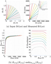 |
Fig. 2 Measured magnetic field strength for unidirectional polarization from 0.1 T up to 1.6 T with a frequency of 50 Hz. |
3 Anisotropic anhysteretic algebraic model
By means ofinterpolation between measured magnetizing curves in different angles, an anhysteretic algebraic model to represent the magnetizability, depending on excitation angles and amplitudes is developed [11]. Figure 3 reveals the model reactions to unidirectional B excitations up to 1.6 T. As the model is based directly on measurements, the simulated anhysteretic H loci behaves closely to the measurements. For lower magnetizations under 1.6 T, the hard magnetization direction rotates from TD to quasi 70°. The black lines represent the amplitude ofB excitations from 0.1 T to 1.6 T. The corresponding H responses are shown also with black lines in H-Loci. At higher magnetization such as 2 T, there is no increase in polarization due to collinearity of domain direction to the applied field direction. The material at this saturation state demonstrates a more isotropic phenomenon as in Figure 4.
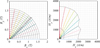 |
Fig. 3 Simulated H-Loci with the anhysteretic anisotropic material model under unidirectional magnetic flux density excitations up to 1.6 T. |
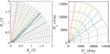 |
Fig. 4 Graphical illustration the magnetic properties with the anhysteretic anisotropic material model under unidirectional magnetic flux density excitations until 2 T. |
4 Hysteresis model
In electrical machines, laminated soft magnetic cores exhibit hysteresis losses. The hysteresis losses are the consequence of sudden jumps of the magnetic domain walls (Barkhausen effect) on microscopic scale as declared in Section 1, these phenomena can be covered through a coupled dynamic constitutive model, as presented in [12] or a pragmatic two-scale model [13]. However, the demand on computation time and memory requirements of these models are enormous. The PAM utilizes an algebraic approximation of a fully coupled lamination model [13], which is based on mesoscopic and is more efficient than dynamic hysteresis model. The stop model can solve microscopic phenomena with a macroscopic view. In this paper, the measured quasi-static major hysteresis loops in RD as commonly indicated as (x) and TD (y), which is depicted in Section 2 with unidirectional excitations, were used to identify both hysteresis models.
4.1 PAM
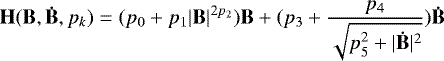
With six parameters in one algebraic formulation equation (1), PAM takes the static and dynamic effects into account. The first term of formulation with parameters p0 − p2 characterizes the anhysteretic magnetization curve. The second term is linked to macroscopic eddy currents. The H is related to the derivative of B with respect to time with parameter p3. The last term with p4 − p5 consideres the hysteresis effect. With the term Ḃ, the hysteresis is interpred in the way of rate dependent.
 (1)
(1)
As the anisotropic character of the material is taken into account, the isotropic scalar PAM equation (1) is extended into a two-dimensional vector hysteresis model [14]. That means the H(B) has a direction dependency and it can be described with Hx(Bx), Hy (By) equation (2). Furthermore, two sets of parameters pk each for x and y directions, need to be determined.
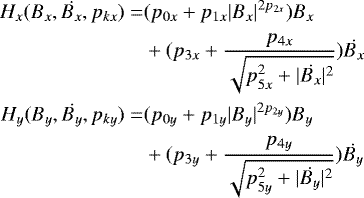 (2)
(2)
By minimizing the least square approximation error between the response of the PAM and the measurements, the identified parameters are summarized in Table 1. The simulated major hysteresis loops by PAM were compared with measured data (Fig. 5). It is apparent that the PAM is capable to represent hysteresis loops with sufficient accuracy. Taking elliptical anisotropy into consideration only twelve parameters need to be determined using two measured major loops. In comparison to anhysteretic anisotropic model, the measurements expense is small. With only one mathematical expression, it ensures a low computation cost compared to play or stop models.
Identified parameters for PAM.
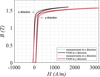 |
Fig. 5 Comparasion of simulated H response by PAM with measured response in RD and TD for FeSi under alternated excitation up to 1.6 T. |
4.2 STOP model
Common hysteresis models have been proposed in the past, such as the well-known Preisach model [15] and Jiles-Atherton model [16]. These models have been vectorized and can offer a precise and continuous representation of rate independent hysteresis of soft magnetic materials. However, it is a challenge to precisely predict the material behavior through extrapolation of measurements. Furthermore, under which condition they satisfy the second law of thermodynamics is still an open question. This paper proposed a quasi-static anisotropic vector stop model inspired by the energy-based model presented in [17]. It is able to display the inverse material constitutive relationship H = H(B) directly with stop operators, avoiding the inversion of play operators which is more efficient from a numerical point of view.
To introduce the stop model, the physical background with respect to the play model is presented firstly. As presented in Section 1, the physical origin of hysteresis at the microscopic level, is on the one hand the anisotropy of crystallites and on the other hand, the Barkhausen jumps caused by pinning forces due to impurities of the materials. According to [18], these domain wall pinning forces are analog to the dry friction forces and its physical explanation, based on thermodynamic potentials, is given as follows.
 (3)
(3)
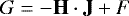
where G corresponds to the Gibb’s energy, F the Helmholz free energy, H the applied magnetic field and J magnetic polarization.
According to the thermodynamic second law, a closed system comes to its steady state by reaching the highest entropy with constant internal energy. This means, a closed system with a constant temperature and pressure takes the state of equilibrium in which its Gibbs free energy has the smallest possible value. The equation (3] can be rewritten as:
 (4)
(4)
The μ as positive definite is deduced by convexity of F. Considering an ideal material without impurities, the material response J to H is a reversible anhysteretic curve. At this state, the corresponding magnetization is denoted as Jre , the magnetic field strength Hre and the free energy Fre. Taking impurities into account, which means the system is discontinued disrupted by small potentials. To overcome these defects in material, an applied magnetic field Hirr must be bigger than the pinning field (slop of these potentials), which in [18] is called as a threshold value k by analogy with a dry friction element. Otherwise, there is no change in J. This causes Barkhausen jumps, which correspond with energy losses hence irreversible process.
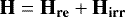
Therefore, the energy potential and magnetic field quantities can be decomposed into reversible and irreversible parts equations (5)–(6). They are the fundamental formulations of the vector hysteresis model proposed in this paper.
 (5)
(5)
 (6)
(6)
The reversible part Hre can be presented as a rheological spring element, which implements a nonlinear anhysteretic character of the material in respect to J. Applying an anisotropy anhysteretic model with this reverserble element, the anisotropy of the stop model can be further improved. The irreversible part Hirr is carried out by a rheological friction slider with a threshold of k. The parallel collection of spring (elastic) and friction slider (perfect plastic) composes a play operator, while the series collection constitutes the stop operator, which both implement the hysteresis effect revealed previously.
Moreover, the pinning force is not homogenized in real material but carried out with a distribution law. A multi-cells model (Prandtl-Ishilinskii’s model) is developed to take this phenomenon into account. Each hysteron possesses a pinning field kn with different amplitudes. As every combination of thermodynamic consistent elements is thermodynamic consistent [19], the Prandtl-Ishilinskii’s model is derived by continuous superposition of play or stop hysterons. As depicted in Figure 6a, the play model with the constitutive relationship J(H) decomposes the polarization J into a finite number n of subfields, while in the stop model, the outcome H is divided into cells.
In contrast to primal models, the stop model (Fig. 6b) has J as the input, and H as the response of the material. Instead of H, the J is divided into a reversible and an irreversible part. Here J, is assumed to be the strain of the rheological elements while H is the stress. As the friction element is combined with spring element in series, the stresses between them are equal to the total stress response of each cell, which means Hre =Hirr=H. Hence, the total H can be evaluated from the spring response Hre from each stop hysterons equation (7).
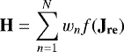 (7)
(7)
here the weight value wn corresponds to the volume density of each hysteron, describing the contribution for the total polarization from each hysteron.
In both models, the anhysteretic nonlinear curve is implemented with the first spring element. The g(Hre) and f(Jre ) are the shape functions each based on play and stop operators.
According to thermodynamics, the hysteresis loops in the form of B(H) should always have a counter-clockwise circular movement due to nonnegative hysteresis dissipation energy. This phenomenon should be revealed by play model. As stop model constituted with H(B), a clockwise movement should be supplied. In order to focus on the main topic of this paper, which is to depict the inverse relationship H = H(B), the play model is not further discussed in details. A geometrically vectorized stop hysteron operator, as equation (8) presented in [20], was applied to the stop model, the scalar model can be directly expanded to a vector model. It is assumed that the difference between polarization of material J and the input magnetic flux density B is neglectable.
 (8)
(8)
with the B0 and  , from previous time point; kn the n-th threshold. The d in
  and Bd means the direction in x or y. Bx and By are the input flux densities in x and y direction. The shape function is based on each stop hysteron constituted. The hyperbolic sine function is used to emulate the shape of H(B) [21]. A graphical representation is depicted in Figure 7. The model is constructed with parallel connection of three cell elements. The first stop hysteron consists of only one elastic spring element which possesses no threshold and is therefore, reversible. This first hysteron represents the anhysteretic nonlinear curve. Increasing the excitation B from zero, the stop hysterons start to rotate clockwise. This means, in Figure 7 the left side of hysterons correspond to the ascending curve and the right side to the descending curve. This represents the thermodynamic consistency as presented previously. For each hysteron, the threshold kn and weight wn are signed.
Furthermore, different kinds of excitations are pushed into a three cells model to test the model’s response. The simulated H-Loci and H(B) curves in each direction are shown in Figure 8.
With three stop hysteron operators, the model is able to reply satisfying results. In the first test case, the excitation B is assumed to rotate (Fig. 8a). The elliptic outcome of H-loci depicts an anisotropy phenomenon of the material.
Next toit, the excitation grows with time (Fig. 8b). The H-loci is denser at lower B and looser at higher flux density excitation. Since B as input increases from zero, the response H rises slower in comparison to B in proximityto the saturation value. This behaves exactly the other way in a play model. In Figure 8c, this three cells model is able to build minor loops for a third ordered harmonic excitation.
The same measurements have been used to test the stop model. Moreover, the same unidirectional field as for the PAM is given as input to the model. The modelled main loops in x and y direction are compared to the measured one. The parameters are identified to minimize the error. With three stop hysteron operators, the validated results are shown in Figure 9. Deviations around the knee of the hysteresis curves are apparent and more significant than in the PAM.
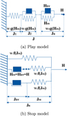 |
Fig. 6 Schematic illustration of the mechanical analogy for energy based multi-cells play and stop models. |
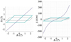 |
Fig. 7 Three stop hysteron operators Sk,x and the shape function f(Bx) with respect to the input magnetic flux density B in x direction. |
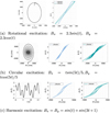 |
Fig. 8 Responses of stop model with three stop hysterons under different excitations. |
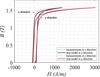 |
Fig. 9 Comparison measured with simulated magnetic fields by stop model. |
5 Numeric experiments
The simulated results are compared to the carried out alternating measurements. The measurements are magnetic flux densities controlled with angles between 0° and 90° and amplitudes between 0 T and 1.6 T. The following figures show the vector responses of the models separated into the x and y direction (Fig. 10).
The anhysteretic model covers the full anisotropy of the material but neglects the hysteretic effect (Fig. 10a). Based on the presented results it can be stated that, with the anisotropic anhysteretic algebraic model, the representation of anisotropy has a good agreement with measurements, but it relates to high measurement efforts. In addition, this is an anhystereticvector model, which neglects the hysteresis effect of electric steel sheets.
The vector hysteretic models PAM and stop can both represent the hysteresis effect. With only two measured major loops in x and y directions, the PAM is able to implement an elliptical anisotropy (Fig. 10b). This means, the vector formulation should be adapted for a better anisotropy, e.g. saturation condition and multiple directions. The static stop model relies on a thermodynamic consistency and its numeric effort is proportional to the number of hysterons. The material responses under a more complicated input signal, for example harmonic excitations, can be reacted with the stop model. In order to validate this excitation, further study will be investigated. By integrating the anhystereticanisotropic model in a stop model, the anisotropy can be more clearly demonstrated (Fig. 10c).
The results are summed up to give an overview and help choosing an appropriate model for the machine design and simulation processes (Tab. 2).
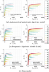 |
Fig. 10 Comparison of models to measurements. |
Comparison of proposed models.
6 Conclusion
This paper utilizes anhysteretic anisotropic model and two different vector hysteresis models. Comparisons to measured data are given. Furthermore, a comparison study with these three models are presented.
The stop model presented here is simplified to update in each time step explicitly. That means the previous time step value is used to update the stop hysterons, which avoids nonlinear iteration and saves computation costs but decreases its accuracy. By means of implicit solving, the model may be improved. A variational approach will be investigated in future works. Another further improvement will deal with the convex energy surface formulation, which directly represents the magnetic anisotropic properties of the material and ensures the numerical robustness of the model.
Acknowledgements
The Deutsche Forschungsgemeinschaft (DFG) within the research project number 373150943 “Vector hysteresis modeling of ferromagnetic materials” supported this work.
Author contribution statement
X. Xiao designed the stop model, carried out the comparison of those models, designed the figures. F. Müller performed the analysis of the Pragmatic Algebraic Model (PAM). Together with X. Xiao and G. Bavendiek he contributed to the interpretation of the results. G. Bavendiek devised the main conceptual ideas, built the anisotropic anhysteretic algebraic model, processed the experimental data and performed the analysis of the data. Prof. K. Hameyer was involved in planning and supervision of the work. All authors provided critical feedback and helped shape the research, analysis and manuscript.
References
- F. Martin, D. Singh, A. Belahcen, P. Rasilo, A. Haavisto, A. Arkkio, Int. J. Comput. Math. Elec. Electron. Eng. 34, 1475 (2015) [CrossRef] [Google Scholar]
- N. Leuning, S. Steentjes, A. Stöcker, R. Kawalla, X. Wei, J. Dierdorf, G. Hirt, S. Roggenbuck, S. Korte-Kerzel, H.A. Weiss et al., AIP Adv. 8, 047601 (2018) [Google Scholar]
- N. Leuning, S. Steentjes, K. Hameyer, IEEE Trans. Magn. 53, 1 (2017) [Google Scholar]
- J. Barros, J. Schneider, K. Verbeken, Y. Houbaert, J. Magn. Magn. Mater. 320, 2490 (2008) [Google Scholar]
- T. Matsuo, M. Shimasaki, IEEE Trans. Magn. 44, 898 (2008) [Google Scholar]
- M. Kuczmann, Physica B 406, 1403 (2011) [CrossRef] [Google Scholar]
- D. Lin, P. Zhou, M. Rahman, A new anisotropic vector hysteresis model based on play hysterons, in 2017 IEEE International Magnetics Conference (INTERMAG) (IEEE, 2017), pp. 1–1 [Google Scholar]
- A. Ramesh, D.C. Jiles, J.M. Roderick, IEEE Trans. Magn. 32, 4234 (1996) [Google Scholar]
- J. Krause, arXiv:1212.5163 (2012) [Google Scholar]
- A. Thul, S. Steentjes, B. Schauerte, P. Klimczyk, P. Denke, K. Hameyer, AIP Adv. 8, 056815 (2018) [Google Scholar]
- G. Bavendiek, N. Leuning, F. Müller, B. Schauerte, A. Thul, K. Hameyer, Arch. Elect. Eng. 68 (2019) [Google Scholar]
- S. Steentjes, F. Henrotte, C. Geuzaine, K. Hameyer, Int. J. Numer. Modell. Electron. Netw. Devices Fields 27, 433 (2014) [CrossRef] [Google Scholar]
- S. Steentjes, F. Henrotte, K. Hameyer, A pragmatic two-scale homogenization technique for ferromagnetic cores at high frequencies, in 9th IET International Conference on Computation in Electromagnetics, 2014, pp. 1–2 [Google Scholar]
- F. Müller, G. Bavendiek, B. Schauerte, K. Hameyer, Arch. Elect. Eng. 68 (2019) [Google Scholar]
- I.D. Mayergoyz, J. Appl. Phys. 63, 2995 (1988) [Google Scholar]
- D.C. Jiles, D.L. Atherton, J. Magn. Magn. Mater. 61, 48 (1986) [Google Scholar]
- V. François-Lavet, F. Henrotte, L. Stainier, L. Noels, C. Geuzaine, J. Comput. Appl. Math. 246, 243 (2013) [Google Scholar]
- A. Bergqvist, Physica B 233, 342 (1997) [CrossRef] [Google Scholar]
- P. Krejcı, Hysteresis, convexity and dissipation in hyperbolic equations (Gakkotosho, Tokyo, 1996) [Google Scholar]
- T. Matsuo, IEEE Trans. Magn. 45, 1194 (2009) [Google Scholar]
- J.V. Leite, N. Sadowski, P. Kuo-Peng, J.P. Bastos, IEEE Trans. Magn. 41, 1500 (2005) [Google Scholar]
Cite this article as: Xiao Xiao, Fabian Müller, Gregor Bavendiek, Kay Hameyer, Analysis of vector hysteresis models in comparison to anhysteretic magnetization model, Eur. Phys. J. Appl. Phys. 91, 20901 (2020)
All Tables
All Figures
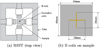 |
Fig. 1 Topology of RSST system [10]. |
| In the text | |
|
Fig. 2 Measured magnetic field strength for unidirectional polarization from 0.1 T up to 1.6 T with a frequency of 50 Hz. |
| In the text | |
|
Fig. 3 Simulated H-Loci with the anhysteretic anisotropic material model under unidirectional magnetic flux density excitations up to 1.6 T. |
| In the text | |
|
Fig. 4 Graphical illustration the magnetic properties with the anhysteretic anisotropic material model under unidirectional magnetic flux density excitations until 2 T. |
| In the text | |
|
Fig. 5 Comparasion of simulated H response by PAM with measured response in RD and TD for FeSi under alternated excitation up to 1.6 T. |
| In the text | |
|
Fig. 6 Schematic illustration of the mechanical analogy for energy based multi-cells play and stop models. |
| In the text | |
|
Fig. 7 Three stop hysteron operators Sk,x and the shape function f(Bx) with respect to the input magnetic flux density B in x direction. |
| In the text | |
|
Fig. 8 Responses of stop model with three stop hysterons under different excitations. |
| In the text | |
|
Fig. 9 Comparison measured with simulated magnetic fields by stop model. |
| In the text | |
|
Fig. 10 Comparison of models to measurements. |
| In the text | |
Current usage metrics show cumulative count of Article Views (full-text article views including HTML views, PDF and ePub downloads, according to the available data) and Abstracts Views on Vision4Press platform.
Data correspond to usage on the plateform after 2015. The current usage metrics is available 48-96 hours after online publication and is updated daily on week days.
Initial download of the metrics may take a while.