| Issue |
Eur. Phys. J. Appl. Phys.
Volume 87, Number 1, 2019
|
|
|---|---|---|
| Article Number | 10501 | |
| Number of page(s) | 9 | |
| Section | Photonics | |
| DOI | https://doi.org/10.1051/epjap/2019190092 | |
| Published online | 06 August 2019 | |
https://doi.org/10.1051/epjap/2019190092
Regular Article
Temporal derivation operator applied on the historic and school case of slab waveguides families eigenvalue equations: another method for computation of variational expressions
1
Université de Rennes, CNRS, Institut de Physique de Rennes − UMR 6251, 35000 Rennes, France
2
Université de Rennes, CNRS, IRMAR – UMR 6625, 35000 Rennes, France
3
Université du Maine, CNRS, Laboratoire d'acoustique de l'Université du Maine − UMR 6613, 72000 Le Mans, France
4
Université de Rennes, CNRS, Institut d'Électronique et de Télécommunications de Rennes − UMR S 6164, 35000 Rennes, France
* e-mail: This email address is being protected from spambots. You need JavaScript enabled to view it.
Received:
19
March
2019
Received in final form:
1
July
2019
Accepted:
15
July
2019
Published online: 6 August 2019
Abstract
Starting from the well-known and historic eigenvalue equations describing the behavior of 3-layer and 4-layer slab waveguides, this paper presents another specific analytical framework providing time-laws of evolution of the effective propagation constant associated to such structures, in case of temporal variation of its various geometrical features. So as to develop such kind of time-propagator formulation and related principles, a temporal derivation operator is applied on the studied school case equations, considering then time varying values of all the geometrical characteristics together with the effective propagation constant. Relevant calculations are performed on three different cases. For example, we first investigate the variation of the height of the guiding layer for the family of 3-layer slab waveguides: then, considering the 4-layer slab waveguide's family, we successively address the variation of its guiding layer and of its first upper cladding. As regards the family of 4-layer waveguides, calculations are performed for two different families of guided modes and light cones. Such another approach yields rigorous new generic analytical relations, easily implementable and highly valuable to obtain and trace all the family of dispersion curves by one single time-integration and one way.
© L. Garnier et al., EDP Sciences, 2019
 This is an Open Access article distributed under the terms of the Creative Commons Attribution License (http://creativecommons.org/licenses/by/4.0), which permits unrestricted use, distribution, and reproduction in any medium, provided the original work is properly cited.
1 Introduction and background
Guided optics has known a considerable evolution since the demonstration of the possibility to guide light by refraction in the mid-nineteenth century by Daniel Colladon [1] and John Tyndall [2]. Both a robust theoretical framework [3,4] and a wide range of technological applications have been developed [5–7]. Concerning the theoretical framework, mainly two kinds of families of waveguide geometries are analytically described by an eigenvalue equation: the pure cylindrical symmetry and the planar symmetry waveguide structures made of several different layers. Most of the other geometries need appropriate approximations (such as the pure Galerkin method or equivalent [8,9], more generally based on spectral method and minimization of residue on approximated functions [10], the Marcatili's method and hybrid one [11,12]), or a step-by-step numerical resolution with a segmentation of the space (multilayer matrix method or finite difference time domain method [13–16] applied on conformal transformation [17,18]). The eigenvalue equations regarding the analytically described geometries are derived by solving the Maxwell's equations in all regions of the global structure, and by properly applying the continuity conditions of the electro-magnetic fields. The opto-geometrical characteristics of the waveguide entail the emergence of a quantification of the modes (called eigenvectors) that can exist within the structure (TE, TM, HE, EH, LP), with indices highlighting the effective number of space-directions being subjected to quantification. For example, the guided modes belong to the light cone of the guiding structure, i.e., in the geometrical optics framework, these modes are coupled with the structure from a region of space allowing total internal reflection inside the structure. Each one of these modes is associated with an effective propagation constant (eigenvalue); the propagation constant is thus directly correlated to the opto-geometrical characteristics of the overall structure (excitation wavelength λ, refractive index of each part of the structure ni
and various spatial geometrical dimensions noted dimi, i integers, Fig. 1). This dependency between dimension and propagation constant is entirely summarized by the dispersion curve associated with the structure. The dispersion curve is a tool valuable in numerous fields of physics and represents the interdependency between two different physical magnitudes of the studied system. In case of guided optics, this dispersion curve provides a link between the effective propagation constant and the previously described opto-geometrical features of the guiding structure (Fig. 1). The correlation between the effective propagation constant and the opto-geometry is highlighted by the above-mentioned eigenvalue equation (or dispersion relation) noted E.v.eq which mathematically corresponds to a functional ℱ of the different parameters of the system: E.v.eq = ℱ (λ, n
i
, dim
i
) here, the different dimi
can be considered either as variables or as fixed parameters). Each set of parameters is associated to a unique family of dispersion curves (Fig. 1); any change of one of these parameters yields a change of the shape of the dispersion curves. The resolution of these eigenvalue equations for a given set of opto-geometrical parameters yields the set of related effective propagation constant β of the optical modes propagating in the structure, which is defined by: (1)with k the vacuum wave number, n
eff the effective refractive index associated to the mode and λ the vacuum wavelength.
(1)with k the vacuum wave number, n
eff the effective refractive index associated to the mode and λ the vacuum wavelength.
In this paper, we theoretically investigate the correlation between the evolution of time-varying geometrical features of families of slab guiding structures and their associated effective propagation constant. To this end, a temporal derivation operator  is applied onto the generic eigenvalue equation regarding the whole family of structures, considering time-dependent values of the studied geometrical dimension (dim ≡ dim(t)) with the effective propagation constant (β ≡ β(t)), and constant values of λ and optical indices. This operation is tantamount to determining a kind of evolution propagator on the eigenvalue equations. Such a way to proceed yields analytical relations shaped as
  enabling to represent the global dynamic displacement along all the family of dispersion curves as geometrical dimensions vary. The time derivation operator (TDO) formulation is performed on the eigenvalue equation of both different essential basic slab-structures: the 3-layer and the 4-layer waveguides. As the eigenvalue equations are derived for constant values of β, we assume that the time variation of the geometrical feature is slow enough to perform an adiabatic evolution treatment. For the 3-layer waveguide (Fig. 2a), we consider a temporal variation of the height noted 2h(t) of the guiding layer. As regards the 4-layer waveguide (Fig. 2b), two cases are considered: firstly, we consider a temporal variation of the height of the guiding layer 2h(t) with a constant height of the first upper cladding 2e(t) before dealing with the opposite situation. For both of these 4-layer cases, the two families of guided modes are investigated [19]. Such an approach should be quite valuable in applied electromagnetism so as to describe numerous processes: for example, while monitoring; a direct layer deposition as a growth process, a processes of sedimentation and soft matter creaming, or etching processes. The results obtained by this model have been compared to COMSOL numerical simulations and show a good agreement.
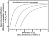 |
Fig. 1 Generic dispersion curves in integrated photonics; each curve is associated with a mode (eigenvector) of a fixed structure at a fixed λ-wavelength. |
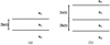 |
Fig. 2 (a) Schematic representation of the 3-layer slab waveguides family; the guiding layer yields a refractive index n 1 and a height 2h, the upper cladding n 3 and the substrate n 4 are both considered as semi-infinite layers. (b) Schematic representation of the family of 4-layer slab waveguides; the index n 1 and n 2 are associated with respectively the guiding layer and the first upper cladding whose height are respectively 2h and 2e. The upper cladding and the substrate of index n 3 and n 4 are considered as semi-infinite layers. |
2 Time derivation formulations and analytical variational expression of eigenvalue equations
2.1 Family of 3-layer slab waveguides
Figure 2a depicts a schematic representation of the family of 3-layer slab waveguides. We consider the layer of index n
1 (n
1 > n
3, n
4) with height 2h ≡ 2h (t) as the guiding layer of such structures. All the effective propagation constants of guided modes thus verify the light's cone n
1 > n
eff
> n
3, n
4. The generic eigenvalue equation ruling all 3-layer slab waveguides is [3,4]: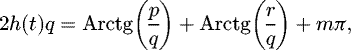 (2)
with
(2)
with  ,
,  ,
,  , h the half height of the guiding layer, and m the order of the considered mode. The optical indices act in the expression of the projection of the wave vector perpendicular to the plane of the layers (considering Pythagoras with a zig-zag geometric-optical ray vision).
We consider the temporal variation of h and relate it to the temporal variation entailed on the effective propagation constant β ≡ β (t). To do so, the above equation is re-written as: (3)
(3)
Then, a temporal derivation operator  is applied in order to express
  in terms of
  . The first step of this calculation allows to compute each derivative of parameters p, q and r, considering time dependent values for β and constant values of k and each ni
(i = 1,3,4).
. The first step of this calculation allows to compute each derivative of parameters p, q and r, considering time dependent values for β and constant values of k and each ni
(i = 1,3,4). (4)
(4)
Then, we can compute the derivatives regarding the arguments as quotients of the Arctg function: (5)
(5)
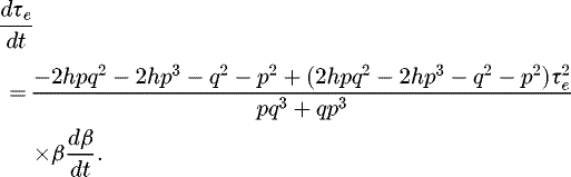
Both varying terms of the numerator of equation (3) may be written as: (6)
(6)
From these calculations, the derivative of the height of the guiding layer comes up as: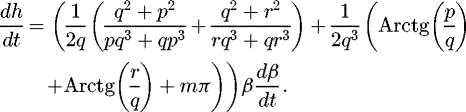 (7)
(7)
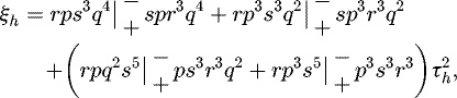
This result can be re-written and formulated as a generic form,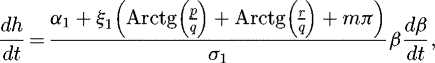 (8)with,
ξ1 = prq4 + pr3q2 + rpq4 + r3p3,
σ1 = 2prq7 + 2pr3q5 + 2rp3q5 + 2r3p3,q3 and β defined in equation (1).
2.2 Family of 4-layer slab waveguides
Considering 4-layer slab waveguides, two cases are dealt with: first, we consider a time dependent value of the height of the guiding layer and a constant value of the height of the first upper cladding (h ≡ h (t)) and e = constante): conversely, we consider the opposite case (h = constante and e ≡ e (t)). For each one of these configurations, two families of guided modes exist: (i) a strongly confined mode with effective index values verifying n
1 > n
eff > n
2 > n
3, n
4 and (ii) a weakly confined one for which n
1 > n
2 > neff > n
3, n
4. Both families may be studied in parallel thanks to a double notation in the following equations: the upper notation
|▪ corresponds to the family of modes verifying condition (i) and the lower one |▪ is related to condition (ii). The structure of a 4-layer slab waveguide is depicted in Figure 2b. The eigenvalue equation describing the behavior of such a waveguide is [18]: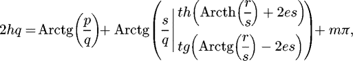 (9)with q, r and p defined the same way as that of the 3-layer waveguide analysis, and
 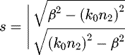 . So as to investigate the effect of any change regarding the height of the guiding layer, equation (9) may be re-written:
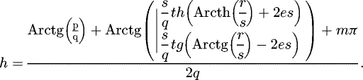 (10)
(10)
The time derivative of q, r and p are given in equation (4), and  verifies:
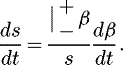 (11)
(11)
This allows us to compute the derivatives of the different ratios: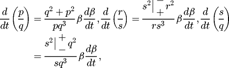 (12)as well as the derivatives of the functions Arctg and Arcth:
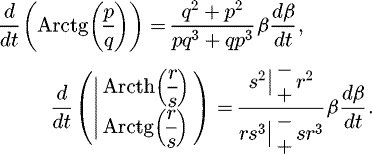 (13)
(13)
To proceed further with the calculations and so as to lighten the expressions, we define: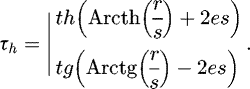 (14)
(14)
Derivating this quantity with respect to time yields: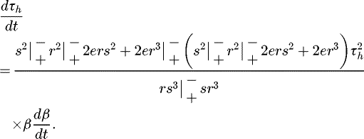 (15)
(15)
Then, we can compute the derivative of the second term of the numerator of equation (11):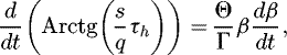 (16)with:
 and
and  .
.
Furthermore, after combining the previous results and simplifying the expressions, the time derivative of the height of the guiding layer is given by: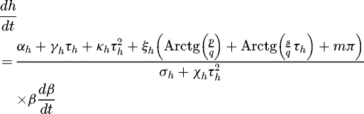 (17)with,


 and β defined in equation (1).
Although equation (11) suits well for the study of the first case (h ≡ h (t)) and e = constante), it comes up as inappropriate for the second one. Then, to study the case e ≡ e (t) and h = constante, it is re-written: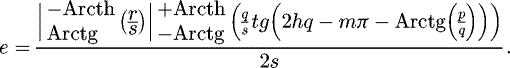 (18)
(18)
Here, so as to find a relation between  and
and  the same methodology as before is applied. We thus compute the time-derivative of the
  ratio:
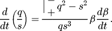 (19)
(19)
Then, we may define a parameter τ
e
before computing its time derivative: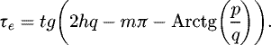 (20)
(20)
 (21)
(21)
Then comes the derivative of the second term of the numerator of equation (18):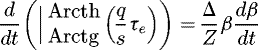 (22)with,

Finally, by combining the previous different results, the time-derivative of e is: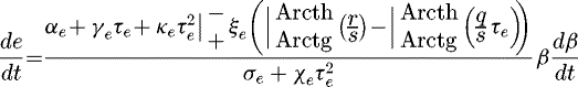 (23)with,


 and β defined in equation (1).
This analysis provides a valuable analytical link between the variation of geometrical features of the global dimensions structures and the correlated changes of all the effective propagation constants describing their associated modes. Each case we have investigated here yields the same generic architecture of relation, yet some significant differences are remarkable. Differences between 3-layer and 4-layer slab waveguides are easily identifiable; they rely on the presence of the factor τ h respectively τ e defined with equation (16) (respectively (20)) also present in the final relation (17) (respectively (23)). Considering the expressions of the variation of the guiding layer of the family of 4-layer slab waveguides for strongly and weakly guided modes, the only differences concern their sign and the expression of τ h . Such sign differences are partially due to the definition of the parameter s whose time derivative only yields unlike signs between the strongly and the weakly guided mode. The other cause of these changed signs is due to both hyperbolic tangent and hyperbolic arctangent functions in the strongly confined mode configuration instead of the conventional tangent and arctangent functions relevant with the weakly confined mode. Naturally, the time derivation of these terms yields only unlike signs. Eventually, the main difference between relations describing time varying guiding layer and time varying first upper cladding is in their dependence as regards the order m of the considered mode. Indeed, in the case of time varying guiding layer this dependency only occurs with the factor noted ξ h conversely, considering the time varying first upper cladding, the order m of the mode is present in the parameter τ e . Hence, the influence of the mode order is more significant in the case of time varying first upper cladding.
3 Numerical implementation and discussion
Numerical implementations of the previous relations have been performed through Matlab programs. These implementations aim at plotting the temporal derivative of the effective index  against time for different sets of opto-geometrical parameters and for different rates of variation of the geometrical features of the structures
  and
and  ). For all the following computations, we consider negative values of
  and
and  , i.e. decreasing values of h and e against time, a wavelength λ = 0.8 µm and only the first mode (m = 0) is investigated.
First, we consider the asymptotic case. Figure 3a represents  against time for a 3-layer slab waveguide and a 4-layer slab waveguide for which 2e → ∞. These two structures yields the same set of parameters (refractive index, initial height of the guiding layer, rate of variation of this height) in order to compare the results in a relevant way. The relative error between these two curves is plotted in Figure 3b. This graph shows that these two cases are numerically equivalent with a maximum relative error below 0.6%. The maximum of relative error occurs at the end of the decrease of the height of the guiding layer, i.e. when 2h is close to the cutting height of the mode.
Let us now investigate the influence of the rate of variation of the geometrical features. To do so, we plot  against time (Fig. 4a) for a 4-layer structure yielding a variation of the height 2h of the guiding layer, for three different values of the rate
  . The other parameters are the initial value of the height of the guiding layer 2h
(t=0 s) = 1 µm, the height of the first upper cladding 2e
(t=0 s) = 0.4 µm and the set of indices (n
1; n
2; n
3; n
4) = (2; 1.8; 1; 1.5). The plot of Figure 4 clearly yields that the ratio between the different values of
. The other parameters are the initial value of the height of the guiding layer 2h
(t=0 s) = 1 µm, the height of the first upper cladding 2e
(t=0 s) = 0.4 µm and the set of indices (n
1; n
2; n
3; n
4) = (2; 1.8; 1; 1.5). The plot of Figure 4 clearly yields that the ratio between the different values of  is equal to the ratio between the corresponding
  which is easily predictable from equation (17). Concerning the values of the times at which the mode disappear, their ratio is equal to the inverse of the ratio between the corresponding
  . In addition, a simulation under COMSOL on a specific structure corroborates this slope, this time considering two close structures to calculate the rate of change Δn
eff (Fig. 4b and Tab. 1).
. In addition, a simulation under COMSOL on a specific structure corroborates this slope, this time considering two close structures to calculate the rate of change Δn
eff (Fig. 4b and Tab. 1).
The influence of the set of indices is investigated in Figures 5a and 5b, which represent the evolution of  against time for a 4-layer structure yielding varying value of the height of the first upper cladding, for strongly and weakly guided mode, respectively. The parameters taken for this simulation are 2h
(t=0 s) = 0.4 µm, 2e
(t=0 s) = 1 µm,
against time for a 4-layer structure yielding varying value of the height of the first upper cladding, for strongly and weakly guided mode, respectively. The parameters taken for this simulation are 2h
(t=0 s) = 0.4 µm, 2e
(t=0 s) = 1 µm, 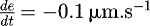 and the investigated set of indices are (n
1; n
2; n
3; n
4) = (2; 1.5; 1; 1) ; (2; 1.8; 1; 1.5); (2; 1.8; 1.5; 1.5). We can see from the graph that the more the mode is confined (great difference between the values of indices) the more abrupt is the slope. Another remarkable property is that the red curve begins to increase before the blue one, which begins to increase before the black one. The reason is that the evanescent part (strongly confined mode) or the oscillating part (weakly confined mode) present in the n
2 layer is more sensitive to the index n
3 in the red curve case because the difference n
2 − n
3 is greater. Concerning the black curve, as the difference n
1 − n
2 is greater than for the other two cases, there is less energy in the n
2 layer so the influence of the n
3 layer is weaker. Similarly, simulations under COMSOL prove the correspondence in terms of variation of the eigenvalue as the dimensions of the structure change (Figs. 5c and 5d and Tab. 2).
and the investigated set of indices are (n
1; n
2; n
3; n
4) = (2; 1.5; 1; 1) ; (2; 1.8; 1; 1.5); (2; 1.8; 1.5; 1.5). We can see from the graph that the more the mode is confined (great difference between the values of indices) the more abrupt is the slope. Another remarkable property is that the red curve begins to increase before the blue one, which begins to increase before the black one. The reason is that the evanescent part (strongly confined mode) or the oscillating part (weakly confined mode) present in the n
2 layer is more sensitive to the index n
3 in the red curve case because the difference n
2 − n
3 is greater. Concerning the black curve, as the difference n
1 − n
2 is greater than for the other two cases, there is less energy in the n
2 layer so the influence of the n
3 layer is weaker. Similarly, simulations under COMSOL prove the correspondence in terms of variation of the eigenvalue as the dimensions of the structure change (Figs. 5c and 5d and Tab. 2).
The TDO formulation starts from an initial condition, defining a starting point in the eigenvalue equation (that is a starting opto-geometric structure), then it deploys its evolutionary principle by giving access to the variation of the eigenvalue when the dimensions of the structure changes over time.
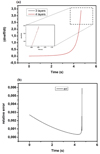 |
Fig. 3 Asymptotic case. (a) Plot of |


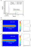 |
Fig. 4 (a) Plot of |


Compared results of the variation of the eigenvalues Δn eff with our variational method based on time derivation operator (TDO), that is, equation (17) and Figure 4, and COMSOL software. As an example, this opto-geometric guiding structure is chosen at fixed parameters: optical indices ( n 1; n 2; n 3; n 4) = (2; 1.8; 1; 1.5), wavelength λ = 0.8 μm and 2e fixed = 0.2 μm, with 2h = 0.4 μm.
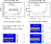 |
Fig. 5 (a) Plot of |


Compared results of the variation of the eigenvalues Δn eff with our variational method based on time derivation operator (TDO), that is equation (23) and Figures 5a and 5b, and COMSOL software. As an example, the opto-geometric guiding structure is chosen at fixed parameters: optical indices ( n 1; n 2 ; n 3; n 4) = (2 ; 1.8 ; 1; 1.5),wavelength λ = 0.8 μm and 2h fixed = 0.4 μm, with dimension 2e = 0.2 μm.
4 Conclusion
This work presents the derivation of generic and rigorous analytical expressions evaluative in time regarding the propagation constant for various families of slab waveguides in case of temporal variation of their geometrical characteristics.
Since the theoretical framework presented in this article hinges on analytical expressions, it provides a valuable tool, easily implementable for numerical computation in one way. Graphically, these expressions are interpretable as a temporal displacement along all the family of dispersion curves of the investigated versatile structures and modes; computing their integral along time obviously leads to the original and generic eigenvalue equations (2) and (9), which gives all the families of dispersion curves (Fig. 1). Their physical meaning, based on the link between  and
and  put them up as specific evolution laws of the propagation constant during any growth or deposition process or during an attack or etching process as regards shaping a given structure. Thus, a direct in situ monitoring becomes possible during thin layer deposition processes in ultra-high-vacuum chambers. The analysis has been performed with 3-layer and 4-layer slab waveguides. In the latter case, the investigation has been carried out for both the variation of the guiding layer and of the first upper cladding, and for the two different families of guided modes. The results computed by the proposed TDO method have been compared to numerical calculations obtained via COMSOL simulations and are in good agreement. Dynamics and therefore evolution are intrinsically contained in the TDO formulation, with the possibility of obtaining a whole family of structures at one time. The advantage brought by this TDO model compared to other numerical simulations, besides that it provides analytical expressions that contain the dynamic, resides in the fact that the other numerical simulations can only resolve static structures, step by step. The simulations have thus to be performed at every time step which take a great amount of time, whereas the proposed TDO formulation (Eqs. (8), (17) and (23)) can be implemented on a regular computer via Matlab or Python, for example, and give results within a few seconds. Furthermore, in a theoretical view, an extended and comprehensive study could be performed in order to determine the overall dynamics of the effective propagation constants in case of the temporal variation of both the above-mentioned layers at the same time. By considering the temporal variation of both 2h(t) and 2e(t) in the 4-layer family waveguides, the time-derivation of equations (10) and (18) should lead to a system of two coupled equations whose resolution should be equivalent to the displacement associated with a set of 2D dispersion maps vision instead of a set of 1D dispersion curves. This model is valid not only for dielectric materials, but also in the presence of a metallic layer, as the eigenvalue equations from which our expressions have been derived are valid whatever the material (see Sect. 2.5 of Ref. [3]). In the case of the presence of a metallic layer, when plasmonic waves can establish, one must take into account the imaginary part of the permittivity ε = (n + iK)2 of the metal. The value of n
2 used in the calculations has thus to be modified to (n
2–K
2) in order to describe the physical behavior of a waveguide comprising a metallic layer, including the propagation of plasmonic waves. Extended studies should also be performed in order to investigate the influence of the temporal variation of the opto-geometrical parameters of more complex photonic structures such as rib waveguide, optical fiber, slab waveguide of an arbitrary large number of layers and metal layers.
put them up as specific evolution laws of the propagation constant during any growth or deposition process or during an attack or etching process as regards shaping a given structure. Thus, a direct in situ monitoring becomes possible during thin layer deposition processes in ultra-high-vacuum chambers. The analysis has been performed with 3-layer and 4-layer slab waveguides. In the latter case, the investigation has been carried out for both the variation of the guiding layer and of the first upper cladding, and for the two different families of guided modes. The results computed by the proposed TDO method have been compared to numerical calculations obtained via COMSOL simulations and are in good agreement. Dynamics and therefore evolution are intrinsically contained in the TDO formulation, with the possibility of obtaining a whole family of structures at one time. The advantage brought by this TDO model compared to other numerical simulations, besides that it provides analytical expressions that contain the dynamic, resides in the fact that the other numerical simulations can only resolve static structures, step by step. The simulations have thus to be performed at every time step which take a great amount of time, whereas the proposed TDO formulation (Eqs. (8), (17) and (23)) can be implemented on a regular computer via Matlab or Python, for example, and give results within a few seconds. Furthermore, in a theoretical view, an extended and comprehensive study could be performed in order to determine the overall dynamics of the effective propagation constants in case of the temporal variation of both the above-mentioned layers at the same time. By considering the temporal variation of both 2h(t) and 2e(t) in the 4-layer family waveguides, the time-derivation of equations (10) and (18) should lead to a system of two coupled equations whose resolution should be equivalent to the displacement associated with a set of 2D dispersion maps vision instead of a set of 1D dispersion curves. This model is valid not only for dielectric materials, but also in the presence of a metallic layer, as the eigenvalue equations from which our expressions have been derived are valid whatever the material (see Sect. 2.5 of Ref. [3]). In the case of the presence of a metallic layer, when plasmonic waves can establish, one must take into account the imaginary part of the permittivity ε = (n + iK)2 of the metal. The value of n
2 used in the calculations has thus to be modified to (n
2–K
2) in order to describe the physical behavior of a waveguide comprising a metallic layer, including the propagation of plasmonic waves. Extended studies should also be performed in order to investigate the influence of the temporal variation of the opto-geometrical parameters of more complex photonic structures such as rib waveguide, optical fiber, slab waveguide of an arbitrary large number of layers and metal layers.
Author contribution statement
Bêche and Gaviot developed the idea of this method (called TDO method) and procedure based on the introduction of a time managing the evolution of electromagnetic structures and thus the course of dispersion curves; they have supervised such project and worked on the manuscript. Garnier performed all the analytical calculation plus the associated simulations; he drafted the manuscript. Doliveira and Mahé simulated under COMSOL to corroborate the previous TDO results.
References
- J.D. Colladon, C.R. Acad. Sci. 15 , 800 (1842) [Google Scholar]
- J. Hecht, City of Light: The Story of Fiber Optics (Oxford University Press, Oxford, 1999) [Google Scholar]
- M.J. Adams, Introduction to Optical Waveguides (John Wiley & Sons, Chichester, 1981) [Google Scholar]
- A.W. Snyder, J.D. Love, Optical Waveguide Theory (Kluwer Academic Publishers, Dordrecht, 2000) [Google Scholar]
- A. Yariv, Quantum Electronics , 2nd edn. (John Wiley & Sons, Chichester, 1957) [Google Scholar]
- T. Tamir, Guided-Wave Optoelectronics , 2nd edn. (Springer-Verlag, Berlin, 1990) [CrossRef] [Google Scholar]
- D. Marcuse, Theory of Dielectric Optical Waveguides (Academic Press, New York, 1974) [Google Scholar]
- D. Marcuse, IEEE J. Quant. Electron. 28 , 459 (1992) [CrossRef] [Google Scholar]
- R.L. Gallawa, I.C. Goyal, Y. Tu, K. Gharak, IEEE J. Quant. Electron. 27 , 518 (1991) [CrossRef] [Google Scholar]
- P.N. Robson, P.C. Kendall, Rib Waveguide Theory by the Spectral Index Method Research , (Studies Press Ltd., New York, 1990) [Google Scholar]
- E.A.J. Marcatili, Bell Syst. Techn. J. 48 , 2071 (1969) [Google Scholar]
- T. Begou, B. Bêche, N. Grossard, J. Zyss, A. Goullet, G. Jézéquel, E. Gaviot, J. Opt. A: Pure Appl. Opt. 10 , 053310.1 (2008) [CrossRef] [Google Scholar]
- M. Koshiba, K. Hayata, M. Suzuki, Electron. Lett. 18 , 411 (1982) [Google Scholar]
- B. Bêche, J.F. Jouin, N. Grossard, E. Gaviot, J. Zyss, Sens. Actuators Phys. A 114 , 59 (2004) [CrossRef] [Google Scholar]
- P. Yeh, A. Yariv, C.-S. Hong, J. Opt. Soc. Am. 67 , 423 (1977) [Google Scholar]
- K.H. Schlereth, M. Tacke, IEEE J. Quant. Electron. 26 , 627 (1990) [CrossRef] [Google Scholar]
- M. Heiblum, J. Harris, IEEE J. Quantum Electron. 11 , 75 (1975) [Google Scholar]
- L. Garnier, C. Saavedra, R. Castro-Beltran, M.J.L. Lucio, E. Gaviot, B. Bêche, Optik 142 , 536 (2017) [Google Scholar]
- B. Bêche, E. Gaviot, A. Renault, J. Zyss, F. Artzner, Optik 121 , 188 (2010) [Google Scholar]
Cite this article as: L. Garnier, A. Doliveira, F. Mahé, E. Gaviot, B. Bêche, Temporal derivation operator applied on the historic and school case of slab waveguides families eigenvalue equations: another method for computation of variational expressions, Eur. Phys. J. Appl. Phys. 87, 10501 (2019)
All Tables
Compared results of the variation of the eigenvalues Δn eff with our variational method based on time derivation operator (TDO), that is, equation (17) and Figure 4, and COMSOL software. As an example, this opto-geometric guiding structure is chosen at fixed parameters: optical indices ( n 1; n 2; n 3; n 4) = (2; 1.8; 1; 1.5), wavelength λ = 0.8 μm and 2e fixed = 0.2 μm, with 2h = 0.4 μm.
Compared results of the variation of the eigenvalues Δn eff with our variational method based on time derivation operator (TDO), that is equation (23) and Figures 5a and 5b, and COMSOL software. As an example, the opto-geometric guiding structure is chosen at fixed parameters: optical indices ( n 1; n 2 ; n 3; n 4) = (2 ; 1.8 ; 1; 1.5),wavelength λ = 0.8 μm and 2h fixed = 0.4 μm, with dimension 2e = 0.2 μm.
All Figures
|
Fig. 1 Generic dispersion curves in integrated photonics; each curve is associated with a mode (eigenvector) of a fixed structure at a fixed λ-wavelength. |
| In the text | |
|
Fig. 2 (a) Schematic representation of the 3-layer slab waveguides family; the guiding layer yields a refractive index n 1 and a height 2h, the upper cladding n 3 and the substrate n 4 are both considered as semi-infinite layers. (b) Schematic representation of the family of 4-layer slab waveguides; the index n 1 and n 2 are associated with respectively the guiding layer and the first upper cladding whose height are respectively 2h and 2e. The upper cladding and the substrate of index n 3 and n 4 are considered as semi-infinite layers. |
| In the text | |
|
Fig. 3 Asymptotic case. (a) Plot of |
| In the text | |
|
Fig. 4 (a) Plot of |
| In the text | |
|
Fig. 5 (a) Plot of |
| In the text | |
Current usage metrics show cumulative count of Article Views (full-text article views including HTML views, PDF and ePub downloads, according to the available data) and Abstracts Views on Vision4Press platform.
Data correspond to usage on the plateform after 2015. The current usage metrics is available 48-96 hours after online publication and is updated daily on week days.
Initial download of the metrics may take a while.