| Issue |
Eur. Phys. J. Appl. Phys.
Volume 83, Number 2, August 2018
Numelec 2017
|
|
|---|---|---|
| Article Number | 20902 | |
| Number of page(s) | 7 | |
| Section | Physics of Energy Transfer, Conversion and Storage | |
| DOI | https://doi.org/10.1051/epjap/2018170420 | |
| Published online | 23 October 2018 | |
https://doi.org/10.1051/epjap/2018170420
Regular Article
A semi-analytical method to compute the magnetic flux linkage of a 2D meshed coil in presence of magnetic materials − application to electrical motor pre-design★
1
Univ. Grenoble Alpes, CNRS, Grenoble INP, G2Elab,
38000
Grenoble, France
2
Altair Motorering,
15 chemin de Malacher,
38340
Meylan, France
* e-mail: This email address is being protected from spambots. You need JavaScript enabled to view it.
Received:
15
December
2017
Received in final form:
6
March
2018
Accepted:
17
August
2018
Published online: 23 October 2018
Abstract
This paper provides a semi-analytical approach for computing the flux linkage of a 2D meshed coil in presence of a non-linear magnetic material. First, a method for flux computation is introduced given the field obtained thanks to a volume integral method. Second, an analytical method for computing the magnetic source field and magnetic vector potential induced by a 2D meshed coil is presented, those quantities being necessary for the flux computation. Comparisons to the finite elements methods are carried out to conclude on the performances of the new method presented.
Contribution to the topical issue “Numelec 2017”, edited by Adel Razek
© EDP Sciences, 2018
 This is an Open Access article distributed under the terms of the Creative Commons Attribution License (http://creativecommons.org/licenses/by/4.0), which permits unrestricted use, distribution, and reproduction in any medium, provided the original work is properly cited.
1 Introduction
One of the key physical quantities while designing an electrical motor [1,2] is the flux linkage of the inductors since it allows to compute the back electromotive force [3,4]. To do so, the finite elements method (FEM) is widely used at an industrial level (see pre-design softwares such as Flux Motor issued by Altair motorering). The FEM yields fairly good results but the computation time can sometimes be a bit long in a pre-design objective [5]. While the FEM needs the whole geometry to be meshed (air, active materials, sources, etc…), the volume integral method (VIM) only requires the meshing of active materials. For a few years, the VIM has been widely studied [6–8] and is know today as a good alternative to the FEM for solving magnetostatic problems in the presence of non-linear materials thanks to the robust acceleration method for its resolution. The magnetic field in the magnetic materials will thus be computed thanks to a 2D VIM presented in [9]. Consequently, the information regarding the magnetic field outside of the active materials is unavailable without an expensive post computation. It is thus necessary to use a flux computation method that requires only the information in the active materials. The method for the flux computation is inspired from [10] and adapted in 2D. This method will be tested with the calculation of the flux linkage of the first phase of a three-phased synchronous permanent magnet electrical motor. The results are compared to those obtained with the FEM.
2 Flux computation method
The flux computation method proposed is complementary to the VIM since it only requires the magnetic field inside the active materials. The vector potential can be split into A = A0 + Am where A0 is the vector potential created by the coils in the vacuum and Am is the vector potential in the magnetic regions. The magnetic flux linkage of a coil k associated to a domain Ω0k can be expressed as [10]:
 (1)
where j0k is the current density vector that creates a current of 1 A in the coil k. Φ0k is the contribution of all coils and Φmk is the contribution of the magnetized part. Let us calculate the contribution of the flux coming from A0. One can write A0 as:
(1)
where j0k is the current density vector that creates a current of 1 A in the coil k. Φ0k is the contribution of all coils and Φmk is the contribution of the magnetized part. Let us calculate the contribution of the flux coming from A0. One can write A0 as:
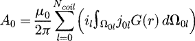 (2)
(2)
with G(r) the 2D Green kernel:  , with r distance between the source point and the target point of integration. The contribution from the coils to the flux linkage of the coil k is:
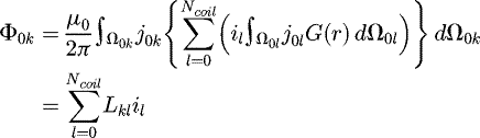 (3)
(3)
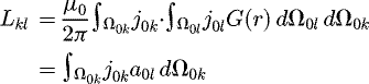
where il is the current through the coil l and:
 (4)
(4)
where a0l represents the vector potential generated by the coil l in the vacuum with a 1 A current and Lkl the self (for k = l) and mutual inductance of the coils in the vacuum.
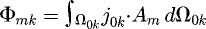
The contribution from the magnetic parts can be written as:
 (5)
that can be modified by the divergence theorem:
(5)
that can be modified by the divergence theorem:
 (6)where H0k is the magnetic field created by the coil k when crossed by a 1 A current, Γ0k is the boundary of the domain Ω0k. The second part of equation (6) is equal to zero since the potential and magnetic field are conserved through Γ0k [10]. We can thus obtain:
 (7)that can be transformed into [10]:
 (8)where Ωm represents the active materials domain and M is the magnetisation. We finally obtain a general formula for the flux linkage of a coil k:
 (9)
(9)
One can notice that the formula necessitates only the information of the magnetic field in the active materials (Ωm). This makes this formula highly compatible with the VIM. Nevertheless, the vector potential and the magnetic field created by the coils are required in the formula (9). The second part of this paper introduces an analytical method to obtain those values.
3 Magnetic field and vector potential induced by a 2D meshed coil
Since the shape of the coils within an electrical rotating machine are not basic shapes (e.g. squares, circles), computing the magnetic field and vector potential generated by those coils is not easy. We have adopted a semi-analytical approach that consists on meshing the inductors with triangles and computing analytical magnetic field and vector potential per triangle Figure 1. Contrary to the 3D situation where Urankar's formulas are well known [11–14], There are no analytical formulas for the field and potential created by a triangle in 2D. Let T be a triangle of the mesh, we can shift and rotate this triangle so that it is in a reference frame (longest edge along the Ox axis) and cut it in two rectangle triangles (see Fig. 2). We can thus compute analytically the field and vector potential created by both triangles T1 and T2 (see Figs. 2 and 3). We could have chosen to work with a normalised reference triangle and a geometrical Jacobian transformation [15] but our approach is more straightforward and easier to implement, that is why we decided to present it here. Moreover, the use of a jacobian transformation is less effective regarding the computation time since more mathematical operations are required for the computation of the field and potential created by each triangle. We use the complex potential created by each triangle defined as [16]:
 (10)
where Ω is the triangle surface crossed by a current density J and z the complex coordinate of the target point. From this potential can be extracted the magnetic field and vector potential:
(10)
where Ω is the triangle surface crossed by a current density J and z the complex coordinate of the target point. From this potential can be extracted the magnetic field and vector potential:
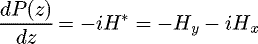 (11)
(11)
 (12)where i is the imaginary number.
Let us compute the complex potential created by T1 and T2 described in Figure 3. The formula for the complex potential yields:
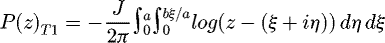 (13)
(13)
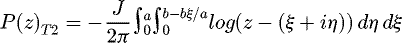 (14)
(14)
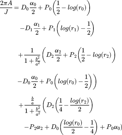
Let us focus on the potential created by T1. We use the fact that a primitive of log(u) is u[log(u) − 1]:
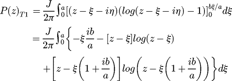 (15)
which leads to, with z0 = 0, z1 = a, z2 = a + ib:
(15)
which leads to, with z0 = 0, z1 = a, z2 = a + ib:
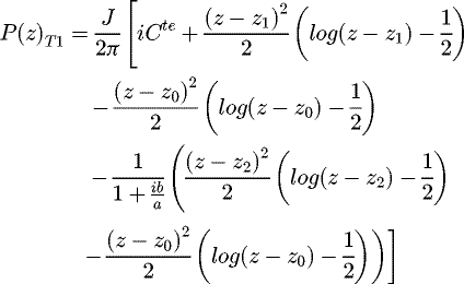 (16)
(16)
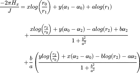
We then use the equations given in equation (11) to get the vector potential:
 (17)
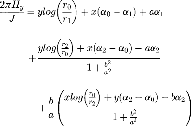
where Di = (y − yi) 2 − (x − xi) 2, and Pi = (x − xi) (y − yi). For the magnetic field:
(17)
where Di = (y − yi) 2 − (x − xi) 2, and Pi = (x − xi) (y − yi). For the magnetic field:
 (18)
(18)
 (19)
(19)
The analytical formulas for the vector potential and the field created by T2 are obtained the same way:
 (20)
(20)
 (21)
(21)
 (22)
(22)
Thanks to those formulas, it is possible to compute the magnetic field and vector potential created by any unspecified triangle and thus by any 2D triangularly meshed coil. Consequently, those formulas allow us to compute the flux with the semi-analytical equation (9).
 |
Fig. 1 Example of the meshed the coil of an electrical motor. |
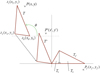 |
Fig. 2 Shifting and rotation of the triangle T. |
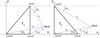 |
Fig. 3 Parametrization of the two rectangle triangles. |
4 Validation of the analytical formulas
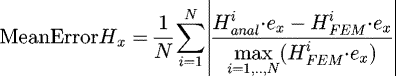
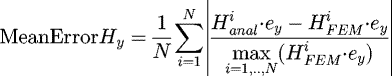
We validate our analytical formulas with the test case presented Figure 4. It consists of three triangularly shaped coils with a current of 1000 A and we computed the field and vector potential along the curve C. We compared the values obtained with our analytical approach to an FEM solution: We plotted the mean;1; difference between the analytical solution and the solution yielded by the FEM for several mesh qualities:
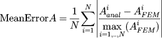 (23)
where N is the number of points along the curve C (we chosed N = 360). The results are displayed Figure 5. The graph shows that the better the FEM problem is meshed, the closer its solution is to the analytical solution, which validates our analytical formulas. The reader can notice that the error on the potential vector is an order of magnitude less than on the magnetic field. This can be explained by the relative “smootheness” of the potential vector due to the fact that it is a primitive to the magnetic field.
(23)
where N is the number of points along the curve C (we chosed N = 360). The results are displayed Figure 5. The graph shows that the better the FEM problem is meshed, the closer its solution is to the analytical solution, which validates our analytical formulas. The reader can notice that the error on the potential vector is an order of magnitude less than on the magnetic field. This can be explained by the relative “smootheness” of the potential vector due to the fact that it is a primitive to the magnetic field.
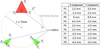 |
Fig. 4 Description of test case. |
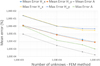 |
Fig. 5 Results of the test case. |
5 Flux calculation in the vacuum
Since the integration of Φ0k is semi-analytical (a0l is computed analytically with the formula described above), we decide to use an adaptative number of Gauss points to ensure the convergence of the calculation, which mean we stop increasing the number of Gauss points when the variation of the flux is less than a certain value (in this paper this value is 0.001%). This allows us to use the coarsest mesh for the coils and still get an accurate value for mutual and self inductances Lkl in equation (4).
We use the algorithm shown Figure 6 to do the calculation, where  is the value of the mutual inductance between coil k and coil l computed with a number of Gauss points i on the Ω0k domain. We used a value of 10−5 for ε. One has to keep in mind that the further the two coils are from each other, the less Gauss points the calculation needs.
To validate our flux in vacuum computation method, we compute the flux in the coil B of the test case Figure 7 with our adaptative semi-analytical method. To validate our approach we use an FEM reference solution, obtained with a sufficiently fine mesh (around 300 000 second order elements). The FEM yielded a value of the flux of 1.792688 × 10⁻⁵ Wb while our adaptative computation yielded 1.792684 × 10⁻⁵ Wb (less than 3 × 10⁻⁵% error). We plot Figure 8 the relative error and the computation time of our adaptative approach for several numbers of Gauss points. We can see that we used 25 Gauss points, computing the result in less than 0.05 s. To obtain this level of precision with the FEM, at least 10 s and a very refined mesh (200 000 elements and 3 gauss points per elements, almost as refined as our “reference solution”) are required while we used only 18 triangles Figure 8.
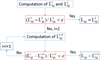 |
Fig. 6 Algorithm for the computation of the inductances. |
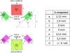 |
Fig. 7 Test case for the flux computation in the vacuum. |
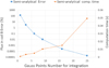 |
Fig. 8 Error and computation time for several Gauss points number used for integration. |
6 Flux computation through the phase of an electrical motor
In order to validate our flux computation method, we used a 24 slot − 8 poles permanent magnet electrical motor (see Fig. 9). We calculated the flux in the phase A of the motor with no current in the coils for several positions of the rotor (from 0 to π/4). Three qualities of mesh have been used for the resolution of the magnetostatic problem via the VIM: 70, 205 and 371 unknowns for one anti-periodicity of the motor. A comparison between the 70 and 371 unknowns mesh can be found Figure 10.
We compared the solution obtained by our flux computation method with one solution obtained via the FEM with a very high quality mesh (around 400 000 elements). The plot of those four curves (one for the FEM reference and three for our method at different qualities of mesh) can be found Figures 11 and 12 while the relative differences between the reference and our method can be found Figure 13. The plot of the computation times required for the FEM and the VIM and the analytical method approach can be found Figure 14.
One can notice that even with a very low number of unknowns, our semi-analytical method yields very accurate results for a very reduced amount of calculation: indeed, while the mean difference between the FEM reference and the solution obtained with 70 unknowns is 2.28% with a maximum difference of 3.81%, the computation time is less than 0.3 s per position of the rotor. This low computation time makes this method very effective in a pre-design context (which was the aim of this study). In opposite, the FEM takes at least 1.5 s per position for the same level of precision (we used a 5000 elements mesh) compared to the reference.
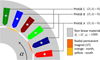 |
Fig. 9 Test case for the flux computation. |
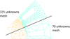 |
Fig. 10 A total of 70 and 371 unknowns mesh for the used for the flux computation. |
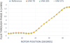 |
Fig. 11 Flux linkage of the phase A of the test motor for several positions of the rotor. |
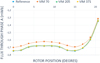 |
Fig. 12 Flux linkage of the phase A of the test motor for several positions of the rotor (zoomed). |
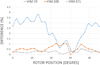 |
Fig. 13 Difference between the reference and the semi-analytic solution for several positions of the rotor. |
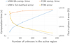 |
Fig. 14 Error and computation time of FEM and VIM + the proposed semi-analytical approach (per position for the computation time). |
7 Conclusions
Original analytical formulas for the computation of the magnetic field and the potential created by a 2D unspecified triangle have been introduced. Those formulas have been rigorously validated with a Finite Elements model. They allow us to calculate semi-analytically the flux linkage of a 2D meshed coil of any shape. This semi-analytical method of flux computation is very well suited for the post processing of a solution yielded by a VIM. We thus used the coupling of the VIM and the proposed method to compute the flux linkage of the phase of a permanent magnet synchronous electrical motor. This coupling allows to gather good quality results rather quickly compared to the FEM. We can see that in addition to being as precise as the FEM for normally meshed problems [7,8,17] is very efficient in a pre-design context, which was the aim of this study.
Author contribution statement
The vast majority of the work has been carried out by Quentin Debray who was then a PhD student under the direction of Dr. Gerard Meunier (Univ. Grenoble Alpes, CNRS, Grenoble INP) and supervised by Dr. Olivier Chadebec (Univ. Grenoble Alpes, CNRS, Grenoble INP), Dr. Jean Louis Coulomb (Univ. Grenoble Alpes, CNRS, Grenoble INP) and Dr. Anthony Carpentier (Altair Engineering). Nevertheless, Drs. Meunier, Chadebec, Coulomb and Carpentier played an essential role of counseling during both the research and redaction phase.
References
- A.O. Di Tommaso, F. Genduso, R. Miceli, Tenth International Conference on Ecological Vehicles and Renewable Energies (EVER) (Monte Carlo, 2015), pp. 1–7 [Google Scholar]
- J. Pythonen, T. Jokinen, V. Hrabovcova, Design of Rotating Electrical Machines (Wiley Editions, 2009) [Google Scholar]
- S.G. Min, B. Sarlioglu, IEEE Trans. Magn. 53, 1 (2017) [CrossRef] [Google Scholar]
- R. Imamura, T. Wu, R.D. Lorenz, Design of variable magnetization pattern machines for dynamic changes in the back-EMF waveform, in Energy Conversion Congress and Exposition (ECCE) (IEEE, 2017) [Google Scholar]
- I. Farmaga, P. Shmigelskyi, P. Spiewak, L. Ciupinski, 11th International Conference The Experience of Designing and Application of CAD Systems in Microelectronics (CADSM) (2011) pp. 213–214 [Google Scholar]
- G. Meunier, O. Chadebec, J.M. Guichon, IEEE Trans. Magn. 51, 1 (2015) [CrossRef] [PubMed] [Google Scholar]
- V. Le-Van, G. Meunier, O. Chadebec, J.M. Guichon, IEEE Trans. Magn. 51, 1 (2015) [CrossRef] [PubMed] [Google Scholar]
- A. Carpentier, O. Chadebec, N. Galopin, G. Meunier, B. Bannwarth, IEEE Trans. Magn. 49, 1685 (2013) [CrossRef] [Google Scholar]
- Q. Debray, G. Meunier, O. Chadebec, J.L. Coulomb, A. Carpentier, IEEE Trans. Magn. 54, 1 (2018) [CrossRef] [Google Scholar]
- L. Huang, G. Meunier, O. Chadebec, J.M. Guichon, Y. Li, Z. He, IEEE Trans. Magn. 53, 1 (2017) [Google Scholar]
- L. Urankar, IEEE Trans. Magn. 16, 1283 (1980) [CrossRef] [Google Scholar]
- L. Urankar, IEEE Trans. Magn. 18, 911 (1982) [CrossRef] [Google Scholar]
- L. Urankar, IEEE Trans. Magn. 18, 1860 (1982) [CrossRef] [Google Scholar]
- L. Urankar, IEEE Trans. Magn. 26, 1171 (1990) [CrossRef] [Google Scholar]
- R. Graglia, IEEE Trans. Antennas Propag. 35, 662 (1987) [CrossRef] [Google Scholar]
- E. Durand, Magnetostatique, Vol. 1 (1968) [Google Scholar]
- V. Le-Van, G. Meunier, O. Chadebec, J.M. Guichon, IEEE Trans. Magn. 52, 1 (2016) [CrossRef] [Google Scholar]
Cite this article as: Quentin Debray, Gerard Meunier, Olivier Chadebec, Jean-Louis Coulomb, Anthony Carpentier, A semi-analytical method to compute the magnetic flux linkage of a 2D meshed coil in presence of magnetic materials − application to electrical motor pre-design, Eur. Phys. J. Appl. Phys. 83, 20902 (2018)
All Figures
|
Fig. 1 Example of the meshed the coil of an electrical motor. |
| In the text | |
|
Fig. 2 Shifting and rotation of the triangle T. |
| In the text | |
|
Fig. 3 Parametrization of the two rectangle triangles. |
| In the text | |
|
Fig. 4 Description of test case. |
| In the text | |
|
Fig. 5 Results of the test case. |
| In the text | |
|
Fig. 6 Algorithm for the computation of the inductances. |
| In the text | |
|
Fig. 7 Test case for the flux computation in the vacuum. |
| In the text | |
|
Fig. 8 Error and computation time for several Gauss points number used for integration. |
| In the text | |
|
Fig. 9 Test case for the flux computation. |
| In the text | |
|
Fig. 10 A total of 70 and 371 unknowns mesh for the used for the flux computation. |
| In the text | |
|
Fig. 11 Flux linkage of the phase A of the test motor for several positions of the rotor. |
| In the text | |
|
Fig. 12 Flux linkage of the phase A of the test motor for several positions of the rotor (zoomed). |
| In the text | |
|
Fig. 13 Difference between the reference and the semi-analytic solution for several positions of the rotor. |
| In the text | |
|
Fig. 14 Error and computation time of FEM and VIM + the proposed semi-analytical approach (per position for the computation time). |
| In the text | |
Current usage metrics show cumulative count of Article Views (full-text article views including HTML views, PDF and ePub downloads, according to the available data) and Abstracts Views on Vision4Press platform.
Data correspond to usage on the plateform after 2015. The current usage metrics is available 48-96 hours after online publication and is updated daily on week days.
Initial download of the metrics may take a while.