| Issue |
Eur. Phys. J. Appl. Phys.
Volume 81, Number 1, January 2018
|
|
|---|---|---|
| Article Number | 11102 | |
| Number of page(s) | 14 | |
| Section | Physics and Mechanics of Fluids, Microfluidics | |
| DOI | https://doi.org/10.1051/epjap/2018170340 | |
| Published online | 30 April 2018 | |
https://doi.org/10.1051/epjap/2018170340
Regular Article
Locus of first crystals on the evaporative surface of a vertically textured porous medium
1
LMDC (Laboratoire Matériaux et Durabilité des Constructions), Université de Toulouse, INSAT, UPS,
Toulouse, France
2
Institut de Mécanique des Fluides de Toulouse, IMFT, Université de Toulouse, CNRS,
Toulouse, France
* e-mail: This email address is being protected from spambots. You need JavaScript enabled to view it.
Received:
5
October
2017
Received in final form:
18
December
2017
Accepted:
9
January
2018
Published online: 30 April 2018
Abstract
The evaporation of a saline solution from a heterogeneous porous medium formed by the assembly of a coarse medium column and a fine medium column is studied numerically. We concentrate on the locus of the formation of first crystals on the evaporative surface from the computation of the ion mass fraction distribution at the surface prior to the efflorescence development. Two basic situations considered in previous works, namely the evaporation–wicking situation and the drying situation are considered. The study makes clear that each situation leads to a markedly different locus of the efflorescence formation, except, however, for very high initial salt concentrations. The study emphasizes the key-role of the velocity field induced in the porous domain in the case of the evaporation–wicking situation. In the case of the drying situation, a key aspect lies in the local increase in the ion mass fraction due to the local desaturation, i.e. the local shrinking of the liquid volume containing the ions.
© B. Diouf et al., published by EDP Sciences, 2018
 This is an Open Access article distributed under the terms of the Creative Commons Attribution License (http://creativecommons.org/licenses/by/4.0), which permits unrestricted use, distribution, and reproduction in any medium, provided the original work is properly cited.
1 Introduction
The presence of dissolved salts in solution in porous media is common in natural systems, e.g. [1], as well as in building materials: bricks, concrete, mortar or stones. In the presence of evaporation, this often leads to the precipitation of salt at the surface of the porous medium where it forms efflorescence or inside where it forms subflorescence. This process of evaporation induced salt precipitation has motivated many studies, notably because it can lead to serious damage, i.e. [2–6] and references therein. Physically, this process can be described as a coupled process of evaporation, ion transport, precipitation and, possibly, mechanical effects (deformation, fracturing, scaling, etc.). Whereas situations combining all these phenomena can be regarded as a main goal in relation with damage generation, less involved situations where damage is negligible are also of interest since a sufficient understanding of crystal localization is an essential first step. Also, the study of evaporation of saline solution in porous media is of interest in relation with other applications than civil engineering, such as soil physics, e.g. [7], or CO2 geological storage, e.g. [8].
As illustrated in Figure 1, it is common to distinguish two main types of situation in this context. In the evaporation–wicking situation, the porous sample is permanently supplied with the solution at its base and remains fully saturated by the solution at any time. In the drying situation, the sample is sealed on every side except on the evaporative surface and the liquid saturation, i.e. the volume fraction of the pore space occupied by the liquid, decreases with time. The evaporation–wicking situation can correspond for instance to walls in a basement whereas the drying situation is expected at higher locations of a wall.
Both situations have been studied in previous studies with model systems formed by assemblies of vertical columns of fine materials (lower mean pore size) and coarse materials (greater mean pore size) containing a sodium chloride aqueous solution. A motivation for the consideration of such heterogeneous materials in the context of civil engineering comes for example from the observation of efflorescence at the surface of brick walls as can be seen on the internet (enter “efflorescence brick walls” and look at the images). Efflorescence can be seen either at the surface of the bricks or at the surface of the mortar between the bricks and sometimes at the surface of both materials. Why the efflorescence locus can be diverse must be understood.
In the evaporation wicking situation, the experiments reported in [9] show the formation of the efflorescence on the surface of the fine material with no efflorescence forming at the surface of the coarse material. By contrast, experiments reported in [10,11] and more recently in [12] show that the efflorescence forms at the surface of the coarse material in drying. Although the situation can be subtler depending on the initial salt concentration [11,12], or the size of the particles used to form the coarse porous medium, e.g. [13,14], the accepted state of the art is thus that efflorescence preferentially forms at the surface of the coarse porous medium in drying and at the surface of the fine porous medium in evaporation wicking. However, the mechanism leading to the preferential precipitation on the surface of the fine medium (evaporation–wicking) or the surface of the coarse medium (drying) are not clear. For example, the preferential deposition over the coarse porous medium in drying is discussed in [12] from the consideration of the formation of wet and dry patches at the surface. We believe that a simpler explanation can be proposed. As discussed in various papers, i.e. [9,15–18], a crucial feature in this type of the problem is the velocity field induced in the porous material by the evaporation process. Understanding the velocity field is an important step because the ions in solution are transported up to the surface by the velocity field. As it is classical in porous medium problems, the velocity field can be considered at different scale. For instance, it is important to consider the velocity field at the pore network scale for explaining the phenomenon of discrete precipitation discussed in [17,18]. Here, since the heterogeneities of interest are at the Darcy's scale, it must be sufficient to consider the problem at Darcy's scale, i.e. within the framework of the classical continuum approach to porous media, e.g. [19].
As we shall see, the consideration of the velocity field and the associated ion convective transport is sufficient to explain the formation of the efflorescence on the fine porous medium surface in the evaporation–wicking situation. However, this is not sufficient for the drying situation which requires considering also the ion concentration local increase effect due to the changes in the local saturation.
In summary, the main objective of the papers is to better explain the locus of efflorescence formation on the surface for both the evaporation–wicking and drying situations.
To this end, we first present briefly an experimental illustration. The corresponding experiments are not fundamentally different from experiments presented in previous works, e.g. [9–14]. However, they illustrate the striking difference between drying and evaporation–wicking as regards the locus of efflorescence formation. Then results extracted from numerical simulations for both situations are presented. The objective of the simulations is to compute the ion mass fraction distributions over the surface. The locus of the ion mass fraction maximum on the surface is a direct indication of the locus of the efflorescence formation since crystallization is supposed to occur when a critical ion mass fraction is reached.
The paper is organized as follows. The experimental illustration is presented in Section 2. The Darcy's scale model enabling us to predict the ion mass fraction distributions is presented in Section 3. The numerical simulation results are presented and discussed in Section 4. Conclusions are drawn in Section 5.
 |
Fig. 1 Two situations of evaporation: (a) evaporation–wicking, (b) drying. |
2 Illustrative experiments
As sketched in Figure 1, experiments are performed with a heterogeneous system made of hydrophilic glass beads. The glass bead system is formed by a central column of smaller beads (100–200 µm in diameter) in contact on two lateral sides with two columns of larger beads (400–600 µm in diameter). The lateral extent of central column is Wf = 2 cm. The lateral extent of each coarse medium column is Wc = 4 cm. The height of the porous domain is L = 3.5 cm. The distance between the two vertical walls confining the beads is 1.5 cm. The set-up used to perform the drying and evaporation–wicking experiments is essentially the same as in previous works [15,17,18] and therefore the details are not presented again. The set-up allows controlling the temperature and relative humidity in the enclosure where the samples are placed. The temperature (T) and relative humidity (RH) are 30 °C and 43%, respectively for each experiment. Experiments are performed with a sodium chloride aqueous solution. The initial salt mass fraction in the solution is 15% (the sodium chloride solubility Csat weakly varies with temperature and is equal to 26.4% at 20 °C).
As sketched in Figure 1, the beads are placed in a vessel so that the evaporative surface is located at a distance δ = 15 mm from the top of the vessel. As shown in [18], this ensures that the evaporation flux is uniform over the surface and not affected by edge effects (which can be quite significant when the surface is flush with the vessel rim [15]).
The experiments lead to the images of the sample surfaces depicted in Figure 2. As expected from previous works, efflorescence forms at the surface of the fine porous medium in evaporation–wicking. By contrast, in drying, this is the opposite. The efflorescence forms at the surface of the coarse porous medium.
 |
Fig. 2 Images of top surface of glass bead system, T = 30 °C, RH = 43% at various times during the evaporation process. Comparison between evaporation–wicking and drying. |
3 Numerical modeling
We present in this section the problems governing the ion transport in the porous system prior to the formation of first crystals for both the evaporation–wicking and drying situations. The evaporation flux density j at the surface is assumed to be the same over the surfaces of the coarse and fine media. This is a well-known property of wet porous medium, e.g. [20], where a similar evaporation rate is observed at the surface of packings of spherical beads regardless of their mean size. Consistently with the experiments, both media are considered as hydrophilic.
The computational domain is illustrated in Figure 3. Owing to the obvious right-left symmetry in Figure 2, this type of domain is also representative of the experimental situation leading to the images depicted in Figure 3.
For both the evaporation–wicking and drying situations, a zero ion mass flux condition is imposed along the lateral boundaries (at x = 0 and x = Wf + Wc, ∀z). For simplicity, this condition is not systematically written in what follows. Only the conditions at the bottom and top surfaces are systematically written.
Note also that for simplicity, the variation of water activity, viscosity, surface tension and density with ion mass fraction are not taken into account.
 |
Fig. 3 Computational domain. Ωf and Ωc are the domains corresponding to the fine and coarse media, respectively. |
3.1 Evaporation–wicking
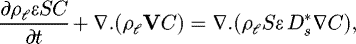
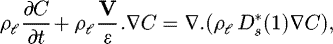
Within the classical framework of the continuum approach to porous media, the equation governing the ion transport in the porous medium reads,
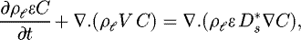 (1)
in which C is the mass fraction of dissolved salt, ϵ is the porosity of the porous medium,
(1)
in which C is the mass fraction of dissolved salt, ϵ is the porosity of the porous medium,  is the effective diffusive coefficient of the dissolved salt in the liquid, V is the filtration (or Darcy) velocity, ρℓ the solution density. The boundary conditions are expressed as:
 (2)
(2)
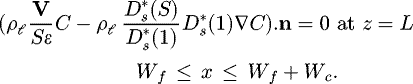
 (3)The zero flux boundary condition (3), where n is the unit vector normal to the considered surface, expresses that the dissolved salt cannot leave the porous medium before the onset of crystallisation. The initial salt mass fraction in the porous domain is uniform and equal to C0, i.e. C = Ci = C0 throughout the sample at t = 0. To solve the above problem, the velocity field in the porous medium must be known. Using Darcy's law, the boundary value problem describing the flow in the porous medium is given by (after decomposition of the pressure according to p = P−ρℓg z),
 (4)
(4)
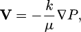 (5)where k is the porous medium permeability and µ the liquid solution viscosity. Equations (4) and (5) are solved subject to the following boundary conditions: P = P0 at z = 0 (P0 ≈ Patm where Patm is the atmospheric pressure), V . n = 0 on the porous domain lateral side (n is here the unit vector normal to the considered lateral boundary). At the porous medium top surface, the evaporation flux j is balanced by the liquid flow coming from the porous medium,
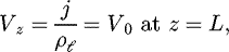 (6)where the evaporation velocity j/ρℓ is denoted by V0. The effective diffusion coefficient is determined according to the relationship
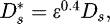 which is classical for granular materials, e.g. [21]; Ds is the ion diffusion coefficient in water (Ds ≈ 1.3 · 10−9 m2/s). Note that the pressure in the liquid phase is actually Pℓ = P − ρℓg (L − z) but we are only interested in the “viscous” contribution P.
The above problem is solved numerically using the commercial simulation software COMSOL Multiphysics.
3.2 Drying
The model for the drying situation is the same as the one presented in [15]. In drying the sample loses water as a result of evaporation and therefore the liquid saturation decreases. A first step is therefore to model the evolution of saturation S; i.e. the local volume fraction of the pore space occupied by liquid. The details on this part of the model can be found in [15].
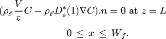
The dissolved salt mass transport within the sample is governed by the following equations,
 (7)
(7)
 (8)
(8)
where V is as before the filtration (Darcy) velocity of the solution. The effective diffusive coefficient of the ions  varies as a function of S according to the relationship
  The zero flux boundary condition (8), which applies to each limiting surface ∂Ω of the porous domain, expresses that the dissolved salt cannot leave the porous medium. The initial ion concentration is denoted by C0 and is spatially uniform.
When all the parameters have been specified, the system formed by equations (7) and (8) and associated boundary and initial conditions is solved numerically together with the problem described in [15] giving the evolution of the saturation and velocity fields using again the commercial simulation software COMSOL Multiphysics.
The zero flux boundary condition (8), which applies to each limiting surface ∂Ω of the porous domain, expresses that the dissolved salt cannot leave the porous medium. The initial ion concentration is denoted by C0 and is spatially uniform.
When all the parameters have been specified, the system formed by equations (7) and (8) and associated boundary and initial conditions is solved numerically together with the problem described in [15] giving the evolution of the saturation and velocity fields using again the commercial simulation software COMSOL Multiphysics.
4 Numerical simulation results (locus of first crystals)
The focus is on the locus of ion mass fraction maximum on the surface and on the mechanisms explaining this locus.
The main parameters for both the evaporation–wicking and drying situations are:
-
the initial mass fraction C0;
-
the height L of the sample;
-
the widths Wf and Wc of the fine and coarse domains;
-
the evaporation flux j = V0ρℓ;
-
the permeability ratio κ = kc/kf.
All simulations are performed with L = 3 cm, Wf = Wc = 0.5 cm assuming granular materials in each column. Unless otherwise mentioned, the average grain diameter is 150 µm in the fine medium and 500 µm in the coarse medium (which corresponds to κ = 11 using the classical Carman-Kozeny relationship). These choices are consistent with the experiments of the literature, e.g. [9–14]. The evaporation flux imposed in the simulation is comparable to the value obtained in the experiments (measured from weighting the sample). We took V0 = 2.07 × 10⁻⁸ m/s. The porosity is expected to be similar in the fine and coarse columns in the glass bead systems but can be different in other heterogeneous systems. For simplicity, we concentrate on the impact on the permeability contrast only. We take εf ≈ εc ≈ 0.36, a typical value for random packings or particles.
Using the classical expression of the Peclet number for this type of problem in the case of an homogeneous sample, e.g. [16],  leads to Pe ≈ 2, which indicates that the ion transport by convection is a key aspect.
For all the simulations, we only consider one value of the initial salt mass fraction, the same as in the experiment, namely C0 = 15%. C0 = 15% is also the salt mass fraction in the bottom reservoir in the evaporation–wicking situation.
Physically, crystallization is expected to occur when the ion mass fraction reaches the critical ion mass fraction Ccr marking the onset of crystallization. As discussed in several works, e.g. [15,22–24], Ccr can be greater than the solubility Csat. However, considering a supersaturation effect would not change the problem under consideration, i.e. the determination of the locus of the ion mass fraction maximum at the surface. However, we do not necessarily stop a simulation when the maximum ion mass fraction reaches a specified value, for example Csat. We actually continue the simulation. This of course can lead to unrealistically high values of the ion mass fraction. It must be realized that the structure of the ion mass fraction field so obtained is actually the same as the one which would have been obtained starting with a lower initial mass fraction (this is so because we neglect the variations of fluid properties with the ion mass fraction). In other words, the evolution of C/C0 is independent of C0. This is obvious from the transport equations. In the same spirit, the fact that the simulations are run for C0 = 15% does not prevent looking at the locus of the ion mass fraction maximum for values lower than Csat. This is in fact fully equivalent to considering the onset of crystallization for a higher initial ion mass fraction.
Note that as in the homogeneous case, a steady state solution is possible in the evaporation–wicking situation whereas this is not possible in drying. However, in drying, we consider situations where the surface of the coarse medium is always well hydraulically connected with the inside of the system (no dry zone forming in the region adjacent to the surface) in accordance with the experimental observations available in the literature.
Although a quantitative comparison with the illustrative experiment is not the objective of the paper, it can be noted that the times computed with the above models when the ion mass fraction reaches the solubility at the surface are 1272 min and 3018 min for the evaporation–wicking and drying cases, respectively. This is in reasonable agreement with the elapsed times before the occurrence of visible crystals in the experiments.
4.1 Evaporation–wicking
The first crystals are observed at the surface of the finer material in the experiments. This is also what is predicted by the continuum model. As depicted in Figure 4, the ion distribution is not uniform at the surface for t > 0. The maximum mass fraction is reached at the left edge of the finer medium surface, at least after a certain elapsed time. For shorter times, the maximum ion mass fraction is still located over the fine medium surface but closer to the interface between the two media. Thus there is a migration of the maximum ion mass fraction locus over a short initial period.
This is so because ions are transported from the coarse region into the fine region in the upper region of the system. It is well known, e.g. [9,18], that the transport of ions and the evolution of the ion mass fraction field is highly dependent of the flow induced in the porous medium under usual conditions, i.e. when the ion convective transport is not small compared to the diffusive transport. The transport is due to the transversal flow field from the coarse medium toward the fine region. This flow field is illustrated in Figure 5. The main features of the flow field can be summarized as follows: (i) the velocity is greater at the inlet in the coarse region; (ii) the flow avoids as much as possible the region of greater hydraulic resistance, i.e. the finer medium; (iii) the flow cannot avoid the finer medium in the top region because of the boundary condition equation (6); (iv) because of point (iii) and as illustrated in Figure 5, stream lines bending occurs in the top region.
 |
Fig. 4 Ion mass fraction distribution at the surface at different times. Distribution of the normalized ion mass fraction |
 |
Fig. 5 Evaporation–wicking: stream lines in the heterogeneous sample (a) with detailed view of velocity field and pressure field (lines of various colors) in the top region of sample (b). Fine column on the left, coarse column on the right. |
4.1.1 Kinematics
Figure 5 makes clear that actually two regions can be distinguished as regards the velocity field: (1) the region away from the surface where the flow is essentially 1D (Vx ≪ Vz) and the velocity is much smaller in the fine region than in the coarse region, (2) the region adjacent to the top surface where the velocity field structure changes significantly compared to the region away from the surface where the velocity field is uniform. To characterize the extent of the top region we define a velocity contrast index as:
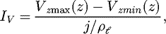 (10)
where Vzmax(z) = max(Vz(x,z)) at z and Vzmin(z) = min(Vz(x,z)) at z. The variation of IV as a function of z is shown in the inset of Figure 6 for two permeability contrast κ = 2 and κ = 10.
(10)
where Vzmax(z) = max(Vz(x,z)) at z and Vzmin(z) = min(Vz(x,z)) at z. The variation of IV as a function of z is shown in the inset of Figure 6 for two permeability contrast κ = 2 and κ = 10.
Figure 6 makes clear that the top zone of velocity reorganization is narrow on the order of Wf (Wf /L = 0.16).
As shown in Appendix, the flow rate at the inlet of each medium can be expressed, respectively, as:
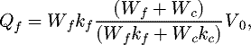 (11)
(11)
 (12)
As a result, the flow rate between the two medium is given by,
(12)
As a result, the flow rate between the two medium is given by,
 (13)which for the special case Wf = Wc yields
Figure 6 shows the variation of Qcf as a function of κ for the case Wf = Wc as predicted by equation (13) together with some numerical computations. The agreement is quite good with the numerical simulations. Note the rapid increase in Qcf with κ. As can be seen, Qcf ≈ V0Wf when the permeability contrast is sufficiently high. Thus, the flow in the fine region away from the top surface is negligible compared to the flow in the coarse region where the mass flow rate is actually equal to the total evaporation rate (i.e. over both the surfaces of the coarse and fine media). As can be seen the flow rate crossing the interface between the two media is independent of the permeability ratio when this ratio is sufficiently high and actually corresponds to the evaporation rate from the fine medium (Qcf ≈ WfV0). Thus in the limit of a sufficiently high permeability contrast, the flow rate corresponding to the evaporation rate from the fine medium is entirely transported within the coarse medium until it is redirected from the coarse medium to the fine medium in the upper region of the system.
 |
Fig. 6 Variation of Qcf/(WfV0) as a function of permeability ratio κ (example for Wf = Wc) as given by equation (17) (solid line). The dashed line with dots corresponds to results obtained from numerical simulations. The inset shows the variation of velocity contrast index IV (Eq. (10)) as a function of z for two permeability contrasts. |
4.1.2 Ion distribution
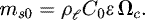
A simple physical explanation for the greater accumulation of ions in the finer porous medium can then be given from the variations of the mass flow rates depicted in Figure 7, namely the mass flow rate Φc of ions entering the medium at the inlet of the coarse medium, the mass flow rate Φf of ions entering (Φf > 0) or leaving (Φf < 0) the medium at the inlet of the fine medium and the mass flow rate Φcf of ions crossing the interface between the two media (with Φcf < 0 when the net transfer is from the coarse to the fine medium). Note that all mass transfer rates in Figure 7 have been made dimensionless by dividing each mass flow rate by Φref = ρℓV0C0Wf.
As can be seen from Figure 7, a quite significant fraction of the ions injected at the inlet of the coarse porous medium is transported toward the finer region owing to the redirection of the flow toward the finer medium.
In the case of the evaporation–wicking situation a steady-state solution can be reached. Figure 7 makes clear that this steady state solution corresponds to a situation where,
 (14)
Thus, the steady state solution is quite different from the steady-state solution for a homogeneous wick, e.g. [18], which is characterized by a zero ion mass flux all along the inlet. In the case of our system, the zero ion mass flow rate at the inlet corresponds to an equilibrium situation where ions enter at the inlet of the coarse medium while the same amount of ions exit the system at the same rate through the fine medium inlet. In other terms, in the steady state regime, ions entering the system through the coarse medium inlet are redirected toward the fine medium inside the system and eventually exit through the fine medium inlet. As depicted in Figure 7, the numerical simulations indicate that the ion mass flow rate entering the system is approximately Φcf ≈ ρℓC0V0Wc in our case.
(14)
Thus, the steady state solution is quite different from the steady-state solution for a homogeneous wick, e.g. [18], which is characterized by a zero ion mass flux all along the inlet. In the case of our system, the zero ion mass flow rate at the inlet corresponds to an equilibrium situation where ions enter at the inlet of the coarse medium while the same amount of ions exit the system at the same rate through the fine medium inlet. In other terms, in the steady state regime, ions entering the system through the coarse medium inlet are redirected toward the fine medium inside the system and eventually exit through the fine medium inlet. As depicted in Figure 7, the numerical simulations indicate that the ion mass flow rate entering the system is approximately Φcf ≈ ρℓC0V0Wc in our case.
The fact that this leads to a greater accumulation of ions into the fine medium can be illustrated from the evolution of the mass gained by each medium until the steady-state is reached. The total mass (per unit length in the y direction) of excess ion injected in the coarse and fine media respectively at time t can be expressed as,
 (15)
(15)
 (16)
(16)
“Excess ion” means in addition to the amount of ions initially present in each column. The variations of Mfex and Mcex are depicted in Figure 8. To end this section on the evaporation–wicking situation, it can be noted that the structure of the velocity field depicted in Figure 5 suggests a simple approximate solution for estimating the steady state ion mass fraction distribution at the surface.
We start from the steady-state solution for a homogeneous medium, e.g. [18] and references therein. This solution reads,
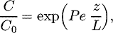 (17)
where
(17)
where  Based on the structure of the velocity field depicted in Figure 5 and the above equation, a simple approximation for the ion mass distribution at the surface is to consider that
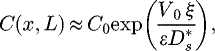 (18)
(18)
where ξ is the length of the stream line connecting the bottom of the sample to the considered point of the surface. From the computation of the stream line lengths, applying equation (18) leads to the distributions shown in Figure 9. The good qualitative agreement with the numerically computed distributions depicted in Figure 9 leads to a simple interpretation in terms of ion transport in a series of stream tubes. The longer is the stream tube connecting the bottom and the top surface, the higher the ion concentration at the corresponding point of the surface.
It is expected that the solution provided by equation (18) will be still better for higher Peclet numbers.
 |
Fig. 7 Evolution of mass flow rates crossing the coarse medium inlet (Φc), entering (Φf > 0) or leaving (Φf < 0) the medium at the fine medium inlet or crossing the interface between the two media (Φcf with Φcf < 0 when the net transfer is from the coarse to the fine medium). Note that all mass transfer rates have been made dimensionless by dividing each mass flow rate by Φref = ρℓV0C0Wc. |
 |
Fig. 8 Variation of Mfex/(Mcex + Mfex) and Mcex/(Mcex + Mfex) as a function of time. |
 |
Fig. 9 Normalized concentration profile at the surface in the evaporation–wicking situation obtained from equation (18) and the computation of streamline lengths. |
4.2 Drying
4.2.1 Kinematics
As illustrated in Figure 10, the drying process is characterized by the preferential desaturation of the coarse medium.
This is an illustration of the well-known capillary pumping effect. The stronger capillary suction in the fine medium induces a flow between the coarse medium and the fine medium allowing the fine medium to stay saturated. This flow is illustrated in the inset of Figure 11. The situation is therefore at first glance similar to the evaporation–wicking situation with a flow from the coarse medium toward the fine medium. It can be noted, however, that the velocity magnitude progressively vanishes with the depth in the drying case (as illustrated in Fig. 11) somewhat as in a homogeneous medium, e.g. [25].
Since there is no desaturation of the fine medium over the considered period, the total flow rate between the two media corresponds to the evaporation rate at the surface of the fine porous medium.
 (19)
where the minus sign indicates that by convention this flow rate is negative when directed from the coarse medium toward the fine one.
(19)
where the minus sign indicates that by convention this flow rate is negative when directed from the coarse medium toward the fine one.
Although this flow rate is constant, the distribution of the velocity along the interface between the two media varies with time, i.e. with the progressive desaturation of the coarse medium. This is illustrated in Figure 11. This is a noticeable difference compared to the evaporation–wicking situation.
Also, there is an interesting change in the velocity direction when a sufficient local desaturation is reached in the coarse medium. The velocity is then directed from the fine medium toward the coarse medium in the upper region of the system. This can be understood by noting that what matters for the flow field is not the intrinsic permeability ratio but the effective permeability ratio
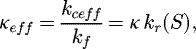 (20)
where the relative permeability in our model, see [15], is expressed as
(20)
where the relative permeability in our model, see [15], is expressed as 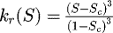 with Sc = 0.1. As a result, the effective permeability decreases in the coarse medium and can become lower than the effective permeability in the fine medium (kfeff = kf) when κ kr(S) < 1. In the case of our simulations κ = 11 and thus κeff < 1 when S < 0.5 in the coarse medium. Since here the desaturation is not uniform owing to gravity effects, saturations lower than 0.5 are first reached in the upper region of the coarse domain, consistently with the inversion in the velocity direction in the upper region of the system depicted in Figure 11. However, this does not necessarily mean that upper region of the fine porous medium starts being invaded by the gas phase. This will happen later but here the net flow rate is still negative (i.e. from the coarse medium to the fine medium) and therefore the fine porous medium stays fully saturated when the change in the velocity direction depicted in Figure 11 is observed. In what follows, we only consider the period of drying when the net flow rate between the two media is negative without any desaturation of the fine porous medium.
 |
Fig. 10 Saturation profile in the coarse medium at various times during drying along the vertical median line in the coarse medium (the saturation varies quite weakly with x in each medium). The inset shows the saturation map at t = 50 h. |
 |
Fig. 11 Profiles of the velocity (normal component Vx) along the interface between the two media (x = Wf) at different times. The velocity is negative when directed from the coarse medium to the fine one. The inset shows the filtration velocity distribution and pressure field (lines of various colors) at two different times (t = 50.3 h on the left, t = 80 h on the right) during the drying process. Fine column on the left, coarse column on the right. |
4.2.2 Ion distribution
Since there is a flow from the coarse porous medium toward the fine one, ions are transported from the coarse porous medium toward the fine one. The ion mass flow rate across the interface between the two media is  (with again by convention Φcf < 0 when the net transfer is from the coarse to the fine medium). The variation of Φcf as a function of time is illustrated in Figure 12. In this figure, ⟨S ⟩ c is the average saturation over the coarse medium.
A naïve view is then to consider that the situation is similar to the evaporation–wicking-situation: ions are transported from the coarse medium to the fine medium and thus the efflorescence must form at the surface of the fine porous medium. However both the experiment (Fig. 2) and the simulation (Fig. 13) show the opposite, at least after a sufficient elapsed time in the simulation. As explained in what follows, this is direct consequence of the preferential desaturation of the coarse medium, a phenomenon specific to drying and which does not happen in the evaporation–wicking situation.
Thus, clearly, the situation in drying is markedly different from the evaporation–wicking situation.
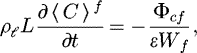
In order to illustrate the key impact of the coarse medium desaturation, let's integrate equations (7) and (8) over the control volumes Ωf and Ωs (see Fig. 5). One obtains,
 (21)
(21)
 (22)
(22)
where  Equations (21) and (22) can be expressed as:
 (23)
(23)
 (24)
(24)
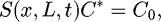
Making for simplicity the approximation 〈SC 〉 c ≈ 〈 S 〉 c 〈 C 〉 c (fully correct for instance when the saturation is uniform in the coarse medium (capillary regime, i.e. [16]) but only an approximation when the saturation varies spatially) leads to express equation (24) as:
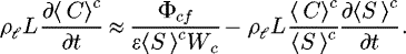 (25)
(25)
The variation of the mean saturation can be deduced from the simple mass balance,
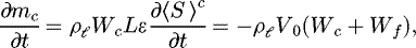 (26)
where mc is the liquid mass in the coarse porous medium (the liquid mass in the fine porous medium does not change, neglecting the variations of density due to the change in salt concentrations, since the desaturation only occurs in the coarse porous medium). Combining equations (25) and (26) yields,
(26)
where mc is the liquid mass in the coarse porous medium (the liquid mass in the fine porous medium does not change, neglecting the variations of density due to the change in salt concentrations, since the desaturation only occurs in the coarse porous medium). Combining equations (25) and (26) yields,
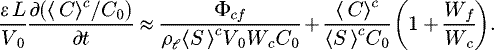 (27)
(27)
Using again Φref = ρℓV0C0Wc as a reference mass flow rate, equation (27) is expressed as:
 (28)
(28)
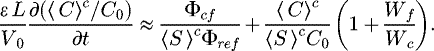
The two terms in the r.h.s. of equation (28) are plotted as a function of time in Figure 12. The results shown in Figure 12 together with equations (23) and (28) make clear the factors affecting the variations of the mean concentration in both media. For the fine medium, the situation is somewhat similar to the evaporation–wicking case. The ion mass fraction increases at the surface as the result of the ion mass flow rate ϕcfcoming from the coarse porous medium and the convective transport toward the surface. The situation is quite different in the coarse porous medium, equation (28), owing to the desaturation effect. As shown in Figure 12, the increase in the average ion mass fraction in the coarse medium originates from the second term in the r.h.s. of equation (28). As can be perhaps seen more explicitly from equation (25), this term is directly related to the desaturation of the coarse medium. The effect is simple. Initially, the coarse medium (of volume Ωc contains the following mass of salt.
 (29)
(29)
Let us neglect here for simplicity the ions transported from the coarse porous medium to the fine one. Then since the salt cannot escape the porous domain, a simple mass balance reads
 (30)
(30)
leading to
 (31)
In the absence of transport, this also holds locally, i.e. C ∝ 1/S. Hence, the greater is the desaturation (i.e. the lower is the saturation), the greater is the ion mass fraction increase. Actually, this effect, referred to as the desaturation effect, takes place together with the transport of ions toward the evaporative surface and the transport of ions in direction of the fine porous medium. Figure 12 simply shows that the desaturation effect is the dominant effect as regards the variation of the ion mass fraction in the coarse medium. In other terms, the desaturation effect overcompensates the ion lost toward the fine medium.
(31)
In the absence of transport, this also holds locally, i.e. C ∝ 1/S. Hence, the greater is the desaturation (i.e. the lower is the saturation), the greater is the ion mass fraction increase. Actually, this effect, referred to as the desaturation effect, takes place together with the transport of ions toward the evaporative surface and the transport of ions in direction of the fine porous medium. Figure 12 simply shows that the desaturation effect is the dominant effect as regards the variation of the ion mass fraction in the coarse medium. In other terms, the desaturation effect overcompensates the ion lost toward the fine medium.
Interestingly, it can be also inferred from equations (23) and (24) that the situation is comparable to the evaporation–wicking situation at short times, i.e. when S ∼ 1. At short times, the mechanism of ion transfer from the coarse to the fine porous medium is dominant and this explains why the efflorescence forms on the surface of the fine porous medium in drying when the initial concentration in ions is sufficiently close to the concentration marking the onset of crystallization. This is illustrated in Figure 13 which shows that the locus of the ion mass fraction maximum is at the surface of the fine region at short times. In this respect, the simulation results are consistent with the experimental results reported in [11,12] showing that the efflorescence forms at the surface of the fine medium when the initial ion mass fraction is quite high (corresponding to a short time of first crystal appearance) whereas the locus of efflorescence is on the coarse medium surface when the initial ion mass fraction is lower, consistently with a longer elapsed time before the occurrence of first crystals at the surface.
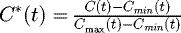
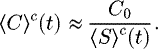
To further illustrate the significance of the desaturation effect at longer times, we can estimate the ion mass fraction at the surface from the simple mass balance (analogous to Eq. (30) but at the surface)
 (32)
where C* denotes the ion mass fraction so obtained.
(32)
where C* denotes the ion mass fraction so obtained.
Using equation (32) at the surface of the coarse medium, an estimator of the average ion mass fraction at the surface of the coarse porous medium can be computed from the saturation distribution at the surface as:
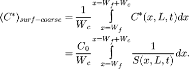 (33)
(33)
In order to assess the impact of the desaturation on the variation of the ion mass fraction we compute the ratio
 (34)
whereCsurf−coarse is the average ion mass fraction at the surface of the coarse porous medium obtained from the numerical solution to the transport problem (Eq. (7)). The variation of Ic is shown in Figure 14 together with the variations of the average saturation over the coarse porous medium as well as at its surface.
(34)
whereCsurf−coarse is the average ion mass fraction at the surface of the coarse porous medium obtained from the numerical solution to the transport problem (Eq. (7)). The variation of Ic is shown in Figure 14 together with the variations of the average saturation over the coarse porous medium as well as at its surface.
As can be seen, the desaturation effect explains here about 80% of the ion mass fraction increase at the surface over the period [30 h–60 h]. If we neglect the ion loss toward the fine medium, which is of negligible influence as regards the ion mass fraction build-up at the surface of the coarse porous medium, two mechanisms contribute to the change in the ion mass fraction at the coarse medium surface. The first one is the desaturation effect as illustrated in Figure 14. The second one is the classical convective transport due to the flow toward the surface induced in the porous medium by the evaporation at the surface. Figure 14 indicates that the first mechanism is dominant over the period [30 h–60 h]. To explain why the second mechanism becomes dominant at longer times, consider the equations governing the ion transports in each medium expressed in non-conservative form as:
Fine medium:
 (35)
(35)
 (36)
Coarse medium:
(36)
Coarse medium:
 (37)
(37)
 (38)The above equations make clear that what matters is the interstitial velocity (V/ε/S). Expressed in dimensionless form and using the same length scale L for both media would lead to define the local effective instantaneous Peclet number in each medium as
  and
and 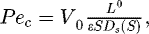 respectively. The ratio between the two Peclet numbers
  is plotted in Figure 15 as a function of saturation.
Thus, the interstitial velocity increases in the coarse porous medium as the result of the decrease in the saturation whereas the effective diffusion coefficient decreases. This leads to greater effective Peclet number in the coarse medium compared to the fine medium. It is known from previous works, i.e. [16,26,27], that the greater the Peclet number is, the faster the increase in the ion mass fraction at the surface. Thus, in addition to the desaturation effect in the coarse medium which causes the increase in the ion mass faction, the greater effective Peclet number in the coarse medium favors a more rapid increase in the ion mass fraction at the surface of the coarse porous medium compared to the fine porous medium. Returning to Figure 14, we thus attribute the significant decrease of IC after 60 h to the increase in the Peclet number induced by the increase in the interstitial velocity, especially in the upper part of the coarse medium.
Integrating over time equations (21) and (22) gives the total mass (per unit length in the y direction) of dissolved salt at time t in the coarse and fine media, respectively,
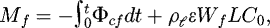 (39)
(39)
 (40)
where we have taken into account the additional constraint that in drying the total mass of dissolved salt does not vary with time before the onset of crystallization.
(40)
where we have taken into account the additional constraint that in drying the total mass of dissolved salt does not vary with time before the onset of crystallization.
The variation of these masses as a function of time is shown in Figure 16. Thus in terms of mass of salt, the fine porous medium gains mass whereas the coarse porous medium loses mass consistently with the existence of a flow from the coarse to the fine porous medium. The somewhat counterintuitive result is that the salt mass loss in the coarse porous medium does not mean a decrease in the ion concentration because the mass loss effect is overcompensated by the desaturation effect.
Finally, in order to further illustrate the key role played by the desaturation effect, we have plotted in Figure 17, the variation of the ratio between the average ion mass fractions at the surface of the coarse and fine media for the nominal case (same evaporation rate at the surface of both media) and when the evaporation rate at the surface of the coarse medium is ten times smaller while the evaporation rate is unchanged at the surface of the fine medium. Figure 18 shows the details of the ion distribution at the surface for the case J = Jref/10, which can be compared with Figure 13 (nominal case).
As a result of the reduction of the evaporation rate at the surface of the coarse medium, the period when the ion mass fraction is greater on the fine porous medium surface is much longer but after a sufficient elapsed time, the ion mass fraction at the coarse porous medium surface becomes much higher than the ion mass fraction at the fine porous medium surface. Since the convective transport of ions toward the surface is severely reduced when J = Jref/10, the preferential increase of the ion mass fraction at the surface of the coarse porous medium is due to the decline in the saturation, i.e. to the desaturation effect.
Finally, the main mechanisms controlling the variation of the ion mass fraction for the two considered evaporation situations are schematically summarized in Figure 19.
 |
Fig. 12 Dissolved salt mass flow rate Φcfthrough the interface between the two media as a function of time (Φref = ρℓV0C0Wc). Variations of the two terms in the r.h.s of equation (28) as a function of time. |
 |
Fig. 13 Distribution of the normalized ion mass fraction |

 |
Fig. 14 Variation IC as a function of time together with the variation of the average saturation in the coarse medium and the average saturation at the surface of the coarse medium (κ = 11). |
 |
Fig. 15 Pec/Pef as a function of S. |
 |
Fig. 16 Variation of Mf /(Mc + Mf) and Mc/(Mc + Mf) as a function of time (κ = 11). |
 |
Fig. 17 Evolution of the ratio between the average ion mass fraction at the surface of the fine medium and at the surface of the coarse one. The inset shows the variation of this ratio when the evaporation rate at the coarse porous medium surface is ten times smaller while the evaporation rate at the surface of the fine medium is unchanged. |
 |
Fig. 18 Distribution of the normalized ion mass fraction |

 |
Fig. 19 Schematic illustration of main mechanisms controlling the variation of the ion mass fraction for the two considered situations. (a) evaporation–wicking, (b) drying. |
5 Conclusion
The occurrence of first salt crystals on the surface of a vertically textured porous medium was studied numerically for both the evaporation–wicking and drying situations. The modelling was based on the classical continuum approach to porous media. The simulations lead to results consistent with the available experimental observations. Ion mass fraction peak forms on the surface of the fine porous medium in the evaporation–wicking situation and on the surface of the coarse porous medium in drying, except at sufficiently short times in drying consistently with the observations that efflorescence forms on the surface of the fine porous medium in drying when the initial ion concentration is sufficiently high [12].
The evaporation–wicking situation and the drying situation should not be mixed up. There are distinct situations leading to distinct results.
In the evaporation–wicking situation, ions are mainly transported within the coarse medium owing to the greater velocity induced in the coarse medium. However, the partial redirection of the flow toward the finer medium in the upper region of the system eventually leads to a greater accumulation of ions in the finer medium. This can be seen as a consequence of the bending of the streamlines in the top region toward the fine porous medium, which leads to longer transport lengths, and thus to greater effective Peclet numbers associated with the ion transport toward the fine region surface. Thus, the study emphasizes the key-role of the velocity field induced in the porous domain on the maximum ion mass fraction locus in the case of the evaporation–wicking situation. Also, the steady-state solution was described and an analytical solution for the flow problem was developed.
The drying case can appear as counter-intuitive at first glance since, as in the evaporation–wicking case, ions are transported from the coarse medium toward the fine one. However, the preferential desaturation of the coarse medium leads to a significant increase in the ion mass fraction since, neglecting here the transport phenomena, the same amount of ions is progressively confined in a smaller and smaller volume of liquid. The result is that the total mass of salt increases in the fine medium (owing to the flux between the two medium) whereas the ion mass fraction increases faster in the coarse medium (owing to the desaturation effect).
Returning to the images of efflorescence on brick walls mentioned in the introduction, formation of efflorescence at the surface of the mortar (finer porous medium) could correspond to evaporation–wicking situations whereas the formation of efflorescence on the brick surface (coarser porous medium) could correspond to a drying situation. Also, it can be surmised that the pore sizes in the mortar are not always necessarily smaller than in the brick. Based on our results, this could also explain the variety of situations observed on brick walls. In this respect, our study allows predicting the most likely place of efflorescence formation from the pore size distributions of both materials.
Appendix
The flow rate crossing the boundary between the coarse and fine regions can be estimated as follows. Sufficiently away from the top surface the pressure only depends on z (thus is independent of x) and is the same in both media. Let us denote this pressure by P*.
Thus the flow rate (per unit length in the y direction) in the fine and coarse regions away from the top interface can be expressed as
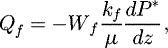 (A.1)
(A.1)
 (A.2)
Since the velocity is known on the top surface (Vz = V0 = j/ρℓ), expressing the flow rate conservation reads
(A.2)
Since the velocity is known on the top surface (Vz = V0 = j/ρℓ), expressing the flow rate conservation reads
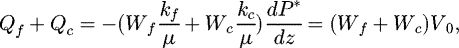 (A.3)
(A.3)
leading to
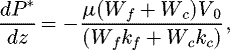 (A.4)
and
(A.4)
and
 (A.5)
(A.5)
 (A.6)
(A.6)
References
- A. Goudie, H. Viles, Salt Weathering Hazards (1997) [Google Scholar]
- C. Noiriel, et al., Chem. Geol. 269, 197 (2010) [Google Scholar]
- G.W. Scherer, Cem. Concr. Res. 29, 1347 (1999) [Google Scholar]
- G.W. Scherer, Cem. Concr. Res. 34, 1613 (2004) [Google Scholar]
- J. Desarnaud, D. Bonn, N. Shahidzadeh, Sci. Rep. 6, 30856 (2016) [CrossRef] [PubMed] [Google Scholar]
- A. Naillon, P. Joseph, M. Prat, Accepted for publication in Physical Review Letters. (2018) [Google Scholar]
- X. Chen, Soil Res. 30, 429 (1992) [CrossRef] [Google Scholar]
- Y. Peysson, Eur. Phys. J. Appl. Phys. 60, 24206 (2012) [CrossRef] [EDP Sciences] [Google Scholar]
- S. Veran-Tissoires, M. Marcoux, M. Prat, Europhys. Lett. 98, 34005 (2012) [Google Scholar]
- M. Bechtold, et al., Geophys. Res. Lett. 38, (2011) [Google Scholar]
- F. Hidri, PhD Thesis, (2013) [Google Scholar]
- M. Bergstad, et al., Water Resour. Res. 53, 1702 (2017) [Google Scholar]
- U. Nachshon, et al., Water Resour. Res. 47, WR010776 (2011) [Google Scholar]
- U. Nachshon, et al., Water Resour. Res. 47, WR009677 (2011) [Google Scholar]
- F. Hidri, et al., Phys. Fluids 25, 127101 (2013) [CrossRef] [Google Scholar]
- H.P. Huinink, L. Pel, M.A.J. Michels, Phys. Fluids 14, 1389 (2002) [CrossRef] [Google Scholar]
- S. Veran-Tissoires, M. Marcoux, M. Prat, Phys. Rev. Lett. 108, 054502 (2012) [CrossRef] [PubMed] [Google Scholar]
- S. Veran-Tissoires, M. Prat, J. Fluid Mech. 749, 701 (2014) [Google Scholar]
- E. Mejri, R. Bouhlila, R. Helmig, Transp. Porous Media 118, 39 (2017) [Google Scholar]
- P. Coussot, Eur. Phys. J. B 15, 557 (2000) [CrossRef] [EDP Sciences] [OGST] [Google Scholar]
- J.-H. Kim, J.A. Ochoa, S. Whitaker, Transp. Porous Media 2, 327 (1987) [Google Scholar]
- J. Desarnaud, et al., J. Phys. Chem. Lett. 5, 890 (2014) [CrossRef] [PubMed] [Google Scholar]
- A. Naillon, et al., J. Cryst. Growth 422, 52 (2015) [Google Scholar]
- A. Naillon, P. Joseph, M. Prat, J. Cryst. Growth 463, 201 (2017) [Google Scholar]
- A.A. Moghaddam, et al., Phys. Fluids 29, 022102 (2017) [CrossRef] [Google Scholar]
- L. Guglielmini, et al., Phys. Fluids 20, 077101 (2008) [CrossRef] [Google Scholar]
- N. Sghaier, M. Prat, S.B. Nasrallah, Transp. Porous Media 67, 243 (2007) [Google Scholar]
Cite this article as: Babacar Diouf, Sandrine Geoffroy, Ariane Abou Chakra, Marc Prat, Locus of first crystals on the evaporative surface of a vertically textured porous medium, Eur. Phys. J. Appl. Phys. 81, 11102 (2018)
All Figures
|
Fig. 1 Two situations of evaporation: (a) evaporation–wicking, (b) drying. |
| In the text | |
|
Fig. 2 Images of top surface of glass bead system, T = 30 °C, RH = 43% at various times during the evaporation process. Comparison between evaporation–wicking and drying. |
| In the text | |
|
Fig. 3 Computational domain. Ωf and Ωc are the domains corresponding to the fine and coarse media, respectively. |
| In the text | |
|
Fig. 4 Ion mass fraction distribution at the surface at different times. Distribution of the normalized ion mass fraction |
| In the text | |
|
Fig. 5 Evaporation–wicking: stream lines in the heterogeneous sample (a) with detailed view of velocity field and pressure field (lines of various colors) in the top region of sample (b). Fine column on the left, coarse column on the right. |
| In the text | |
|
Fig. 6 Variation of Qcf/(WfV0) as a function of permeability ratio κ (example for Wf = Wc) as given by equation (17) (solid line). The dashed line with dots corresponds to results obtained from numerical simulations. The inset shows the variation of velocity contrast index IV (Eq. (10)) as a function of z for two permeability contrasts. |
| In the text | |
|
Fig. 7 Evolution of mass flow rates crossing the coarse medium inlet (Φc), entering (Φf > 0) or leaving (Φf < 0) the medium at the fine medium inlet or crossing the interface between the two media (Φcf with Φcf < 0 when the net transfer is from the coarse to the fine medium). Note that all mass transfer rates have been made dimensionless by dividing each mass flow rate by Φref = ρℓV0C0Wc. |
| In the text | |
|
Fig. 8 Variation of Mfex/(Mcex + Mfex) and Mcex/(Mcex + Mfex) as a function of time. |
| In the text | |
|
Fig. 9 Normalized concentration profile at the surface in the evaporation–wicking situation obtained from equation (18) and the computation of streamline lengths. |
| In the text | |
|
Fig. 10 Saturation profile in the coarse medium at various times during drying along the vertical median line in the coarse medium (the saturation varies quite weakly with x in each medium). The inset shows the saturation map at t = 50 h. |
| In the text | |
|
Fig. 11 Profiles of the velocity (normal component Vx) along the interface between the two media (x = Wf) at different times. The velocity is negative when directed from the coarse medium to the fine one. The inset shows the filtration velocity distribution and pressure field (lines of various colors) at two different times (t = 50.3 h on the left, t = 80 h on the right) during the drying process. Fine column on the left, coarse column on the right. |
| In the text | |
|
Fig. 12 Dissolved salt mass flow rate Φcfthrough the interface between the two media as a function of time (Φref = ρℓV0C0Wc). Variations of the two terms in the r.h.s of equation (28) as a function of time. |
| In the text | |
|
Fig. 13 Distribution of the normalized ion mass fraction |
| In the text | |
|
Fig. 14 Variation IC as a function of time together with the variation of the average saturation in the coarse medium and the average saturation at the surface of the coarse medium (κ = 11). |
| In the text | |
|
Fig. 15 Pec/Pef as a function of S. |
| In the text | |
|
Fig. 16 Variation of Mf /(Mc + Mf) and Mc/(Mc + Mf) as a function of time (κ = 11). |
| In the text | |
|
Fig. 17 Evolution of the ratio between the average ion mass fraction at the surface of the fine medium and at the surface of the coarse one. The inset shows the variation of this ratio when the evaporation rate at the coarse porous medium surface is ten times smaller while the evaporation rate at the surface of the fine medium is unchanged. |
| In the text | |
|
Fig. 18 Distribution of the normalized ion mass fraction |
| In the text | |
|
Fig. 19 Schematic illustration of main mechanisms controlling the variation of the ion mass fraction for the two considered situations. (a) evaporation–wicking, (b) drying. |
| In the text | |
Current usage metrics show cumulative count of Article Views (full-text article views including HTML views, PDF and ePub downloads, according to the available data) and Abstracts Views on Vision4Press platform.
Data correspond to usage on the plateform after 2015. The current usage metrics is available 48-96 hours after online publication and is updated daily on week days.
Initial download of the metrics may take a while.