© M.F. De Andrade Paschoal et al., Published by EDP Sciences, 2025

1 Introduction

A particle, far from any solid boundaries, in a fluid at rest, is subject to gravitational forces due to the density contrast between the particle and the fluid. This density difference drives the particle's motion, and as it moves, it experiences viscous forces from the fluid. In steady-state or creeping flow regimes, the particle is solely subject to these forces and its velocity is constant. This configuration is well-known, particularly in rheology, because understanding the dynamics of a spherical particle allows for a straightforward determination of a Newtonian fluid's viscosity [1–3]. This has even led to the well-known falling-ball viscometer. For practical purpose, the fluid is generally confined within a tube of radius R_t, which affects the drag force on the particle of diameter R_b. This setup has been studied in both Newtonian [1,2,4] and non-Newtonian fluids e.g. [5–9], studies focusing only on the vertical motion of the ball. The measurement of the field of a falling magnet allows to study non-transparent fluids [10]. Non-Newtonian fluids exhibit viscosities that vary non-linearly with flow properties and may also show characteristics like viscoplasticity or viscoelasticity. The key properties for these fluids are yield stress for viscoplastic fluids and elastic and loss moduli for viscoelastic fluids. In these cases, the particle's motion is significantly influenced by the fluid's non-Newtonian properties, making the drag force determination complex. Extensive research has been conducted to develop accurate models. In the present work, we aim to investigate the dynamics of a falling particle enriched by an additional body force. To modify the particle's dynamics [11–13], we propose introducing an electromagnetic force that can counteract gravity within a defined region.

For this purpose, we consider a ring magnet centered on the tube, that interacts with ferromagnetic beads (Fig. 1). The magnetic field of the ring magnet can be understood as the superposition of the fields of two fictitious solid cylindrical magnets of same height H and same symmetry axis, but different radii and opposite magnetic poles (the first, with a radius R_o, has its north pole on the top, whereas the second, with a radius R_i < R_o has its south pole on the top). As a result, the axial magnetic field of the ring magnet is zero at a certain distance of the center of the magnet (≈20 mm for the magnet and bead used). The vertical electromagnetic force on the bead is attractive above this point and repulsive below, modulating the force exerted on the particle [14]. In addition to this vertical modulation, the electromagnetic force has a radial component that becomes strong enough to influence the particle's trajectory as it approaches the magnet, pulling the particle toward the magnet ring. Consequently, the particle may deviate from the tube central axis as it approaches the magnetic ring. This combination of vertical and radial forces makes the particle's dynamics more complex compared to the systems without any magnet. However, the system allows for better control over the particle's motion, resulting in more consistent and repeatable trajectories. This is highly advantageous, as bead trajectories are typically difficult to control when wall effects and non-Newtonian fluids are involved. This configuration also presents the advantage of enabling a controlled investigation of the particle's lateral motion, something that has never been done before. Finally, the wall-effect with the tube must be equally investigated to obtain accurately the drag force as a function of the lateral position [15,16].

A clear understanding of this system requires several key steps: (i) the mathematical formulation of the bead dynamics in a configuration with a ring magnet fixed to the outer tube (Sect. 2), (ii) the determination of the magnetic force exerted by the ring magnet on a magnetizable bead (Sect. 3), and (iii) a rigorous comparison of numerical and experimental results, including magnetic force and bead trajectories, in Newtonian fluids (Sect. 4). Preliminary results for non-Newtonian fluids are presented in Section 5.

Fig. 1 Sketch of falling bead.

2 Trajectories computation

The motion of a ferromagnetic bead (of position ${\displaystyle \overrightarrow{x}}$) in a tube filled with fluid, on which is centered the ring magnet, is described by:

$$m\frac{d^2{\displaystyle \overrightarrow{x}}}{d{t}^2}={{\displaystyle \overrightarrow{f}}}_d+{\displaystyle \tilde{m}}{\displaystyle \overrightarrow{g}}+{\displaystyle \overrightarrow{f}}$$(1)

where m is the mass, ${{\displaystyle \overrightarrow{f}}}_d$ the drag force, ${\displaystyle \tilde{m}}$ the modified mass due to buoyancy, ${\displaystyle \overrightarrow{g}}$ the gravity and ${\displaystyle \overrightarrow{f}}$ the magnetic force. The motion is both vertical (along z) and lateral (along $r=\sqrt{x^2+y^2}$). The unsteady Basset drag and added mass force terms are neglected (acceleration of the fluid and inertial term are not considered due to the motion involved) [17,18].

For Newtonian fluids, when the radius of the tube containing the fluid is infinite, the Stokes formula [19] gives the drag force as:

$${{\displaystyle \overrightarrow{f}}}_d=-6\pi {\mu }_d{R}_b\frac{d{\displaystyle \overrightarrow{x}}}{dt}$$(2)

where µ_d is the dynamic viscosity, R_b the bead radius. If the tube has a finite radius R_t, and if the bead stays on the axis of the tube (r = 0) the Francis correction factor α [2] is introduced in (2) as follows:

$${{\displaystyle \overrightarrow{f}}}_d=-\alpha 6\pi {\mu }_d{R}_b\frac{d{\displaystyle \overrightarrow{x}}}{dt}\text{with}\alpha ={\left(\frac{1-0.475R_b/R_t}{1-R_b/R_t}\right)}^4.$$(3)

If the bead position is not on the axis of the tube (r ≠ 0), the 3D Stokes problem has to be computed to find the real drag force of the bead in the fluid tube. The momentum equation for the fluid in the creeping flow regime is:

$${\mu }_d\text{Δ}{\displaystyle \overrightarrow{u}}-{\displaystyle \overrightarrow{▽}}P={\displaystyle \overrightarrow{0}}$$(4)

(where ${\displaystyle \overrightarrow{u}}$ is the fluid velocity and P the pressure) under the constraint of incompressibility

$${\displaystyle \overrightarrow{▽}\cdot }{\displaystyle \overrightarrow{u}}=0.$$(5)

The strain rate tensor ${\displaystyle \underset{\_}{{\displaystyle \underset{\_}{D}}}}=1/2\left({\displaystyle {\displaystyle \overrightarrow{▽}}\overrightarrow{u}}+t{\displaystyle \overrightarrow{▽}}{\displaystyle \overrightarrow{u}}\right)$ is solution in the fluid domain Ω of

$${\displaystyle \underset{P}{\text{max}}}{\displaystyle \underset{{\displaystyle \underset{\_}{{\displaystyle \underset{\_}{D}}}}}{\text{min}}}{\displaystyle \underset{\Omega }{{\displaystyle \int }}}[{\mu }_d|{\displaystyle \underset{\_}{{\displaystyle \underset{\_}{D}}}}{|}^2-PTr\left({\displaystyle \underset{\_}{{\displaystyle \underset{\_}{D}}}}\right)]d{\displaystyle \overrightarrow{x}}$$(6)

with a prescribed velocity of $d{\displaystyle \overrightarrow{x}}/dt$ on the boundary of the bead ∂D, which is the minimization of the energy dissipation under the constraint of free-divergence velocity [20,21].

The power balance gives the drag force as:

$${{\displaystyle \overrightarrow{f}}}_d\cdot \frac{d{\displaystyle \overrightarrow{x}}}{dt}={\displaystyle \underset{\Omega }{{\displaystyle \int }}}2{\mu }_d|{\displaystyle \underset{\_}{{\displaystyle \underset{\_}{D}}}}{|}^{2}d{\displaystyle \overrightarrow{x}}$$(7)

Then additional correction factors α_r and α_z, depending on (r, R_b, R_t) are added to the Stokes formula (2) respectively for lateral and vertical motions.

The correction factor in the z-direction α_z is almost equal to the correction α proposed by Francis unless the sphere is close to the tube wall (Tab. 1). Concerning the correction factor in the r-direction α_r, we suggest to approximate it by a function (dashed lines in Fig. 2) given by:

$${\alpha }_r\left(r\right)\simeq \alpha {\beta }_0\left[1+{\beta }_1\left(e^{{\beta }_2\frac{r}{R_t}}-1\right)\right].$$(8)

When the bead gets closer to the tube, the increase of friction due to the bead-wall interaction is quantified. The accuracy of the lateral drag force is necessary to get the real trajectory. Finally, for the case of Newtonian fluids, the system of ordinary differential equations which describes the trajectory is:

In following sections, our aim is to determine the forces as functions of the position, including the wall-effects, to compute the trajectories via (9), and then compare them to experimental ones.

In the case of non-Newtonian fluids, such as the yield-stress fluids, the drag force is no longer similar and it has to be evaluated considering the fluid's constitutive equation [9,22].

$$\frac{d}{dt}\left[\begin{array}{l}r\hfill \\ m{\displaystyle \dot{r}}\hfill \\ z\hfill \\ m{\displaystyle \dot{z}}\hfill \end{array}\right]=\left[\begin{array}{l}\hfill {\displaystyle \dot{r}}\hfill \\ f_r\left(r,z\right)-{\alpha }_{r}6\pi R_b{\mu }_d{\displaystyle \dot{r}}\hfill \\ \hfill {\displaystyle \dot{z}}\hfill \\ f_z\left(r,z\right)-{\alpha }_{z}6\pi R_b{\mu }_d{\displaystyle \dot{z}}-{\displaystyle \tilde{m}}g\hfill \end{array}\right].$$(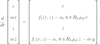9)

Fig. 2 Correction factors (αr, αz) in r and z-directions for various ratio Rt/Rb (dashed lines: approximation function).

3 Magnetic force computation

When ferromagnetic objects are introduced, in the neighbourhood of a magnet, of source field ${{\displaystyle \overrightarrow{h}}}_s$, an induced field is created, and the total field is the sum of the source field and the induced field. Then total induction verifies:

$${\displaystyle \overrightarrow{b}}\left({\displaystyle \overrightarrow{x}}\right)+{{\displaystyle \overrightarrow{b}}}_s\left({\displaystyle \overrightarrow{x}}\right)=\mu \left({\displaystyle \overrightarrow{x}}\right)({\displaystyle \overrightarrow{h}}\left({\displaystyle \overrightarrow{x}}\right)+{{\displaystyle \overrightarrow{h}}}_s\left({\displaystyle \overrightarrow{x}}\right)$$(10)

where ${\displaystyle \overrightarrow{b}}$, ${\displaystyle \overrightarrow{h}}$, µ are respectively the induced induction, the induced magnetic field, and the permeability. The force which acts on the bead, can be obtained by virtual work: the virtual displacement of the ferromagnetic domain is considered to find the force due to the magnet. However, if the ferromagnetic domain moves, then the permeability function changes, which is not the case if the magnet is moved instead. Then, for reasons of simplicity, the choice is made to move the magnet from its initial position labelled 1 with a translation 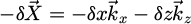$-\delta {\displaystyle \overrightarrow{X}}=-\delta x{{\displaystyle \overrightarrow{k}}}_x-\delta z{{\displaystyle \overrightarrow{k}}}_z$ to a new position labelled 2. The induced magnetic fields corresponding to both positions 1 and 2 are labelled ${{\displaystyle \overrightarrow{h}}}_1$ and ${{\displaystyle \overrightarrow{h}}}_2$. The field difference between ${{\displaystyle \overrightarrow{h}}}_1$ and ${{\displaystyle \overrightarrow{h}}}_2$ verifies:

$$\nabla \cdot [\mu \left({\displaystyle \overrightarrow{x}}\right)({{\displaystyle \overrightarrow{h}}}_2\left({\displaystyle \overrightarrow{x}}\right)-{{\displaystyle \overrightarrow{h}}}_1\left({\displaystyle \overrightarrow{x}}\right))+\left(\mu \left({\displaystyle \overrightarrow{x}}\right)-{\mu }_0\right)({{\displaystyle \overrightarrow{h}}}_s\left({\displaystyle \overrightarrow{x}}+\partial {\displaystyle \overrightarrow{X}}\right)-{{\displaystyle \overrightarrow{h}}}_s\left({\displaystyle \overrightarrow{x}}\right))]=0.$$(11)

The difference of source magnetic fields can be expressed as a Taylor series expansion (up to the second order) as:

$${{\displaystyle \overrightarrow{h}}}_s\left({\displaystyle \overrightarrow{x}}+\partial {\displaystyle \overrightarrow{X}}\right)-{{\displaystyle \overrightarrow{h}}}_s\left({\displaystyle \overrightarrow{x}}\right)\simeq {\displaystyle \overrightarrow{{\displaystyle \overrightarrow{\nabla }}}}{{\displaystyle \overrightarrow{h}}}_s\left({\displaystyle \overrightarrow{x}}\right)\delta {\displaystyle \overrightarrow{X}}+\frac{1}{2}\delta {\displaystyle \overrightarrow{X}}{\displaystyle \overrightarrow{{\displaystyle \overrightarrow{{\displaystyle \overrightarrow{\nabla }}}}}}{{\displaystyle \overrightarrow{h}}}_s\left({\displaystyle \overrightarrow{x}}\right)\delta {\displaystyle \overrightarrow{X}}$$(12)

The field difference between ${{\displaystyle \overrightarrow{h}}}_1$ and ${{\displaystyle \overrightarrow{h}}}_2$ is:

$${{\displaystyle \overrightarrow{h}}}_2-{{\displaystyle \overrightarrow{h}}}_1\simeq {\displaystyle \overrightarrow{{\displaystyle \overrightarrow{\nabla }}}}{{\displaystyle \overrightarrow{h}}}_1\left({\displaystyle \overrightarrow{x}}\right)\delta {\displaystyle \overrightarrow{X}}+\frac{1}{2}\delta {\displaystyle \overrightarrow{X}}{\displaystyle \overrightarrow{{\displaystyle \overrightarrow{{\displaystyle \overrightarrow{\nabla }}}}}}{{\displaystyle \overrightarrow{h}}}_1\left({\displaystyle \overrightarrow{x}}\right)\delta {\displaystyle \overrightarrow{X}}$$(13)

Since the following relationship is verified (D is the domain of the bead):

$${\displaystyle \underset{D}{{\displaystyle \int }}}\left(\mu \left({\displaystyle \overrightarrow{x}}\right)-{\mu }_0\right)({{\displaystyle \overrightarrow{h}}}_s\left({\displaystyle \overrightarrow{x}}+\delta {\displaystyle \overrightarrow{X}}\right)-{{\displaystyle \overrightarrow{h}}}_s\left({\displaystyle \overrightarrow{x}}\right))\cdot {{\displaystyle \overrightarrow{h}}}_1\left({\displaystyle \overrightarrow{x}}\right)d{\displaystyle \overrightarrow{x}}={\displaystyle \underset{D}{{\displaystyle \int }}}\left(\mu \left({\displaystyle \overrightarrow{x}}\right)-{\mu }_0\right){{\displaystyle \overrightarrow{h}}}_s\left({\displaystyle \overrightarrow{x}}\right)\cdot ({{\displaystyle \overrightarrow{h}}}_2\left({\displaystyle \overrightarrow{x}}\right)-{{\displaystyle \overrightarrow{h}}}_1({\displaystyle \overrightarrow{x}})d{\displaystyle \overrightarrow{x}}.$$(14)

The force components can then be computed as:

$$f_i={\displaystyle \underset{D}{{\displaystyle \int }}}\left(\mu \left({\displaystyle \overrightarrow{x}}\right)-{\mu }_0\right){{\displaystyle \overrightarrow{h}}}_s\left({\displaystyle \overrightarrow{x}}\right)\cdot {\partial }_i\left({\displaystyle \overrightarrow{h}}\left({\displaystyle \overrightarrow{x}}\right)+{{\displaystyle \overrightarrow{h}}}_s\left({\displaystyle \overrightarrow{x}}\right)\right)d{\displaystyle \overrightarrow{x}}={\displaystyle \underset{D}{{\displaystyle \int }}}\left(\mu \left({\displaystyle \overrightarrow{x}}\right)-{\mu }_0\right)\left({\displaystyle \overrightarrow{h}}\left({\displaystyle \overrightarrow{x}}\right)+{{\displaystyle \overrightarrow{h}}}_s\left({\displaystyle \overrightarrow{x}}\right)\right)\cdot {\partial }_i{{\displaystyle \overrightarrow{h}}}_s\left({\displaystyle \overrightarrow{x}}\right)d{\displaystyle \overrightarrow{x}}$$(15)

where i stands for (x, y, z), and ${\displaystyle \overrightarrow{h}}={{\displaystyle \overrightarrow{h}}}_1$ is the field of the initial position, and the fields ${\partial }_i{\displaystyle \overrightarrow{h}}$ are computed by:

$$\nabla \cdot \left[\mu \left({\displaystyle \overrightarrow{x}}\right){\partial }_i{\displaystyle \overrightarrow{h}}\left({\displaystyle \overrightarrow{x}}\right)+\left(\mu \left({\displaystyle \overrightarrow{x}}\right)-{\mu }_0\right){\partial }_i{{\displaystyle \overrightarrow{h}}}_s\left({\displaystyle \overrightarrow{x}}\right)\right]=0.$$(16)

The components of the stiffness matrix are:

$$\frac{\partial f_i}{\partial j}={\displaystyle \underset{D}{{\displaystyle \int }}}\left(\mu -{\mu }_0\right)\left[\begin{array}{l}\left({\displaystyle \overrightarrow{h}}+{{\displaystyle \overrightarrow{h}}}_s\right)\cdot {\partial }_{ij}{{\displaystyle \overrightarrow{h}}}_s+{\partial }_i{{\displaystyle \overrightarrow{h}}}_s\cdot {\partial }_j{{\displaystyle \overrightarrow{h}}}_s\hfill \\ +\frac{1}{2}\left({\partial }_i{{\displaystyle \overrightarrow{h}}}_s\cdot {\partial }_j{\displaystyle \overrightarrow{h}}+{\partial }_j{{\displaystyle \overrightarrow{h}}}_s\cdot {\partial }_i{\displaystyle \overrightarrow{h}}\right)\hfill \end{array}\right]d{\displaystyle \overrightarrow{x}}$$(17)

where i and j stand for (x,y,z). The source field ${{\displaystyle \overrightarrow{h}}}_s$ of the ring magnet has a closed-form expression for a constant magnetization, so its derivatives are easily obtained. If the magnetization is not parallel to the axis of the ring, then more elaborate formulas may be found [23]. From a computational point of view, scalar potentials can be introduced to compute ${\displaystyle \overrightarrow{h}}$ and its derivatives. Since the stiffness matrix of the finite element problem is the same (only the right-hand side containing the source induction field and its derivatives changes), a L-U decomposition can be carried out once for all, and the forward-back substitution is done to find ${\displaystyle \overrightarrow{h}}$ and its derivatives.

The magnetic force has to be pre-computed accurately as a function of the position of the bead (r, z) to use it afterwards for the ordinary differential set of equations (9). For a given mesh of (r, z) bead's positions, the use of splines with force derivatives allow a better accuracy.

The force derivative ∂f_z/∂ z exerted on a bead (R_b = 2.17mm), is computed with (17) (Fig. 3) : it is weakly dependent of the lateral position of the bead x, unless the bead is close to the magnet. It allows to find the relative extrema of f_z (z).

The absolute difference between ∂f_z/∂ z obtained by (17) and by numerical differentiation of the force obtained with (15) is computed (Fig. 4) leading to a relative difference of approximately 5–10%.

Figure 5 (on top) highlights the eccentricity effects of the force derivative ∂f_z/∂ x (computed with (17)). The relative difference between the force derivative and its numerical differentiation is in the range of ±10%. The same conclusion can be drawn for ∂f_x/∂ x (bottom of Fig. 5).

To get the force for any point, force components (and their derivatives) are computed for a given rectangular grid of (10×50) equidistant points. Then cubic splines obtained using only the force components, are compared with cubic splines obtained using both the force components and their derivatives. For the same grid, the accuracy of the force components is enhanced with splines obtained using both the force components and their derivatives (Figs. 6 and 7 for a given x = 2.5 mm, not part of the grid and a variable z). On top of each figure, is the finer grid, and on the bottom is the coarser grid. Even with a coarse grid, for both force components, the minimal accuracy is 5% for the splines based on the force derivatives (except when the force is low), whereas the minimal accuracy is beyond 20% for the splines based solely on the force. Similarly, splines based on the force and its derivatives offer improved accuracy at the boundaries compared to those using only the force.

If the field ${{\displaystyle \overrightarrow{h}}}_s$ was uniform, then the magnetization of the spherical bead would be:

$${\displaystyle \overrightarrow{m}}=3\frac{\mu -{\mu }_0}{\mu +2{\mu }_0}{{\displaystyle \overrightarrow{h}}}_s.$$(18)

When the permeability µ of the bead tends towards infinity, then an approximation of the force is:

$${\displaystyle \overrightarrow{f}}\simeq {\mu }_{0}2\pi R_b^3{\displaystyle \overrightarrow{\nabla }}(|{{\displaystyle \overrightarrow{h}}}_s\left({{\displaystyle \overrightarrow{x}}}_b\right){|}^2).$$(19)

The stiffness matrix can also be obtained by:

$${\displaystyle \overrightarrow{{\displaystyle \overrightarrow{\nabla }}}}{\displaystyle \overrightarrow{f}}\simeq {\mu }_{0}2\pi R_b^3{\displaystyle \overrightarrow{{\displaystyle \overrightarrow{\nabla }}}}(|{{\displaystyle \overrightarrow{h}}}_s\left({{\displaystyle \overrightarrow{x}}}_b\right){|}^2)$$(20)

This approximation is all the more valid as the bead radius is low.

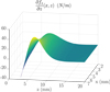Fig. 3 Force derivative $\frac{\partial f_z}{\partial z}$ (in N/m) exerted on a bead (Rb = 2.17 mm) as a function of its position (x, 0, z).

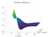Fig. 4 Absolute difference between ∂fz/∂ z obtained with (17) and by numerical differentiation (in N/m).

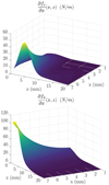Fig. 5 Force derivatives with respect to x (N/m) exerted on a bead (Rb = 2.17 mm) as a function of its position (x, 0, z).

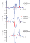Fig. 6 Accuracy of fz for different types of spines (top: finer grid, bottom: coarser grid).

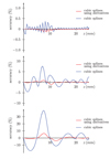Fig. 7 Accuracy of fx for different types of spines (top: finer grid, bottom: coarser grid).

4 Results

A ferromagnetic bead is dropped in the tube filled with glycerol (µ_d = 1 Pa.s) of inner radius R_t = 7 mm. The magnetization of the ring magnet is M = 0.8810⁶A/m: it has been deduced from the measurement of the source field with a Gaussmeter. Its dimensions are : outer radius R_o = 17 mm, inner radius R_i = 12 mm, height H = 10 mm.

The force has been computed and divided by $R_b^3$ to show the validity of the approximated formula: it is a good approximation for radii below 2mm and far from the magnet (Fig. 8). The vertical component is also compared with experiment (for R_b = 2.2 mm).

The force derivative of f_z with respect to z and x has also been divided by $R_b^3$ (Fig. 9). The relative difference between approximation and real value is quite large when the bead is close to the magnet, even when the bead radius is 1mm. The approximated formula only gives an estimate of the real value.

Experiments have been conducted, and several bead's radii (0.4–2.2 mm) were tested. Two cameras recorded experimental (x, z) and (y, z) bead's positions (Fig. 10) as a function of time to reconstruct the (r, z) trajectory.

The ball falls almost at constant r at the beginning and then at almost constant z dividing the trajectory into two main motions (Fig. 11, r = z = 0 is the center of the magnet). First, the magnet attracts the bead vertically, until a close distance to the equilibrium position. Then, the radial motion occurs until the bead stops when reaching the tube wall, which is a stable position for the bead. Up to 0.5 s the position is close to the free fall one (i.e. without magnetic force). The ordinary differential set of equations (9) was solved with an embedded Dormand-Prince 4(5) method. There is a close fit between the computed trajectory and the experimental one, which validates the model.

The computed velocities are also close to the experimental ones (Fig. 12). The free-fall speed (about 18 mm/s) is reached in less than 0.1 s, and then the vertical speed increases due to the magnetic force, and decreases when it changes sign, then the lateral speed rises, and the equilibrium position is reached.

The experimental device allows to find the fluid viscosity by reproducing numerically the experimental trajectories. Figure 13 shows the bead velocities as a function of time with the fluid viscosity µ_d as parameter. The maximum of the velocities ṙ and ż is linear with the inverse of the viscosity, and the times when this maximum occurs is linear with the viscosity. Since maxż and t(maxż) are independent of the initial lateral position, then these measures can be used to find the viscosity. From a practical point of view, with the apparatus we used, the t(maxż) was measured. Then the simulation gives the t(maxż) as a function of the viscosity. Viscosity accuracy is about 6%.

The lateral motion also gives the order of magnitude of the drag force with wall effects. However, more points (than those of the experiments) would be needed to rebuild accurately the drag force from the experiment. When the bead's radius changes (all other parameters are fixed), the maximum of ż varies linearly with the radius (and this maximum is independent of the initial position) (Fig. 14). It is not the case for the maximum of ṙ, since the drag force changes with the ratio R_b/R_t. The times at which the lateral velocities are extremal, vary as $R_b^{-5/3}$ (it is initial position-dependent for ṙ). The total time trajectory is proportional to $R_b^{-3/2}$.

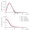Fig. 8 Vertical (top) and lateral (bottom) force divided by $R_b^3$ for several bead radii (black: approximated force with (20), measurements for Rb = 2.2 mm: symbols) as a function of the height.

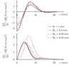Fig. 9 Vertical force derivatives divided by $R_b^3$ for several bead radii (black: approximated force derivative with (20)).

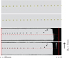Fig. 10 Falling bead with magnetic effect (bottom Rb = 0.8 mm) or without (top Rb = 1 mm).

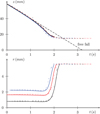Fig. 11 Position of a bead (Rb = 1.45 mm) as a function of time (crosses: experimental, plain lines : numerical) for different starting abscissa positions (black r0 = 0.8 mm, red 1.5 mm, blue 2.2 mm).

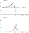Fig. 12 Bead velocities (Rb = 1.45 mm) as a function of time (crosses: experimental, plain lines: numerical) for the same starting abscissa positions (and same color code) as Figure 11 (black r0 = 0.8 mm, red 1.5 mm, blue 2.2 mm).

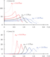Fig. 13 Bead velocities (Rb = 2.17 mm) versus time, with viscosity µd as parameter.

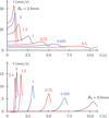Fig. 14 Bead velocities (µd = 1Pas) versus time, with bead radius Rb as parameter.

5 Towards non-Newtonian fluids

The case of Newtonian fluids has been closely investigated to show the accuracy of the computations. The extension to non-Newtonian fluids has also been tested: a Herschel-Bulkley fluid has been used [9]. The relationship between the stress tensor ${\displaystyle \underset{\_}{{\displaystyle \underset{\_}{\tau }}}}$ and the strain-rate tensor ${\displaystyle \underset{\_}{{\displaystyle \underset{\_}{D}}}}$ is:

$$\{\begin{array}{ll}{\displaystyle \underset{\_}{{\displaystyle \underset{\_}{\tau }}}}=\left[\left(n+1\right)k_i|{\displaystyle \underset{\_}{{\displaystyle \underset{\_}{D}}}}{|}^n+{\tau }_y\right]\frac{{\displaystyle \underset{\_}{{\displaystyle \underset{\_}{D}}}}}{\left|{\displaystyle \underset{\_}{{\displaystyle \underset{\_}{D}}}}\right|}\hfill & ,\text{if}\left|{\displaystyle \underset{\_}{{\displaystyle \underset{\_}{\tau }}}}\right|>{\tau }_y\hfill \\ {\displaystyle \underset{\_}{{\displaystyle \underset{\_}{D}}}}={\displaystyle \underset{\_}{{\displaystyle \underset{\_}{0}}}}\hfill & ,\text{if}\left|{\displaystyle \underset{\_}{{\displaystyle \underset{\_}{\tau }}}}\right|\le {\tau }_y\hfill \end{array}.$$(21)

The strain-rate tensor ${\displaystyle \underset{\_}{{\displaystyle \underset{\_}{D}}}}$ is found by:

$${\displaystyle \underset{P}{\text{max}}}{\displaystyle \underset{{\displaystyle \underset{\_}{{\displaystyle \underset{\_}{D}}}}}{\text{min}}}{\displaystyle \underset{\Omega }{{\displaystyle \int }}}[(k_i|{\displaystyle \underset{\_}{{\displaystyle \underset{\_}{D}}}}{|}^n+{\tau }_y)\left|{\displaystyle \underset{\_}{{\displaystyle \underset{\_}{D}}}}\right|-PTr\left({\displaystyle \underset{\_}{{\displaystyle \underset{\_}{D}}}}\right)]d{\displaystyle \overrightarrow{x}}$$(22)

and the drag force is:

$${{\displaystyle \overrightarrow{f}}}_d\cdot \frac{d{\displaystyle \overrightarrow{x}}}{dt}={\displaystyle \underset{\Omega }{{\displaystyle \int }}}{\displaystyle \underset{\_}{{\displaystyle \underset{\_}{\tau }}}}::{\displaystyle \underset{\_}{{\displaystyle \underset{\_}{D}}}}d{\displaystyle \overrightarrow{x}}.$$(23)

The flow index for the experiment is n = 0.49, the consistency index k_i = 0.3Pa.sⁿ, the yield stress τ_y = 0.6Pa. Mainly two types of methods can be used to find the solution of (22). The first is the viscosity regularisation model [9,24], which does not recover the unyielded region but gives a fair value of the drag force. The second is the augmented Lagrangian method [24] which can provide the unyielded regions but is somewhat slow to converge and the value of its parameters is problem-dependant. The value of the drag force in our problem is almost the same with both methods.

Figure 15 shows the trajectories of a bead of radius 0.25mm for various initial positions. The solid lines are the computed trajectories, and the crosses correspond to the experimental points (more experimental points are obtained due to the longer time of the experiment than with the beads of larger diameter). The same kind of trajectory is obtained as for Newtonian fluids : the effects of the magnetic force are the same. The time when the lateral motion occurs is about the same for computation and experiment : it is larger when the initial position of the bead is near the axis.

Figure 16 shows the bead velocities for the same trajectories as Figure 15 (with the same color). Far from the magnet the vertical velocity is the one of the free fall, and does not depend too much of the initial radial position, since the bead diameter is much lower than the tube diameter. It is of the same order of magnitude for a large range of initial radial positions. Computed velocities are close to experimental ones.

Fig. 15 Position of a bead (Rb = 0.25 mm) in a Herschel-Bulkley fluid as a function of time (crosses: experimental, plain lines: numerical) for different starting abscissa positions (black r0 = 0.38 mm, red 3.6 mm, blue 5.0 mm).

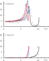Fig. 16 Velocities of a bead (Rb =0.25 mm) in a Herschel-Bulkley fluid as a function of time (crosses: experimental, plain lines: numerical) for the same initial abscissa positions (same color code) as Figure 15 (black r0 = 0.38 mm, red 3.6 mm, blue 5.0 mm).

6 Conclusion

The fall of a magnetic bead in the field of a ring magnet, is first a vertical motion, and then mostly a sideways motion, which is difficult to obtain. The magnetic force has been obtained accurately for any bead position: it allows to reproduce the dynamics of the experiment for Newtonian and non-Newtonian fluids. The next step would be to extract the lateral drag force with the experimental trajectory (by subtracting the other forces), especially when wall effects are predominant, and find working formulas as a function of fluid parameters.

Funding

This research received no external funding.

Conflicts of interest

None.

Data availability statement

The data that support the findings of this study are available from the corresponding author upon reasonable request.

Author contribution statement

Authors equally contributed to the article.

References

All Tables

All Figures

	Fig. 1 Sketch of falling bead.
In the text

	Fig. 2 Correction factors (αr, αz) in r and z-directions for various ratio Rt/Rb (dashed lines: approximation function).
In the text

	Fig. 3 Force derivative $\frac{\partial f_z}{\partial z}$ (in N/m) exerted on a bead (Rb = 2.17 mm) as a function of its position (x, 0, z).
In the text

	Fig. 4 Absolute difference between ∂fz/∂ z obtained with (17) and by numerical differentiation (in N/m).
In the text

	Fig. 5 Force derivatives with respect to x (N/m) exerted on a bead (Rb = 2.17 mm) as a function of its position (x, 0, z).
In the text

	Fig. 6 Accuracy of fz for different types of spines (top: finer grid, bottom: coarser grid).
In the text

	Fig. 7 Accuracy of fx for different types of spines (top: finer grid, bottom: coarser grid).
In the text

	Fig. 8 Vertical (top) and lateral (bottom) force divided by $R_b^3$ for several bead radii (black: approximated force with (20), measurements for Rb = 2.2 mm: symbols) as a function of the height.
In the text

	Fig. 9 Vertical force derivatives divided by $R_b^3$ for several bead radii (black: approximated force derivative with (20)).
In the text

	Fig. 10 Falling bead with magnetic effect (bottom Rb = 0.8 mm) or without (top Rb = 1 mm).
In the text

	Fig. 11 Position of a bead (Rb = 1.45 mm) as a function of time (crosses: experimental, plain lines : numerical) for different starting abscissa positions (black r0 = 0.8 mm, red 1.5 mm, blue 2.2 mm).
In the text

	Fig. 12 Bead velocities (Rb = 1.45 mm) as a function of time (crosses: experimental, plain lines: numerical) for the same starting abscissa positions (and same color code) as Figure 11 (black r0 = 0.8 mm, red 1.5 mm, blue 2.2 mm).
In the text

	Fig. 13 Bead velocities (Rb = 2.17 mm) versus time, with viscosity µd as parameter.
In the text

	Fig. 14 Bead velocities (µd = 1Pas) versus time, with bead radius Rb as parameter.
In the text

	Fig. 15 Position of a bead (Rb = 0.25 mm) in a Herschel-Bulkley fluid as a function of time (crosses: experimental, plain lines: numerical) for different starting abscissa positions (black r0 = 0.38 mm, red 3.6 mm, blue 5.0 mm).
In the text

	Fig. 16 Velocities of a bead (Rb =0.25 mm) in a Herschel-Bulkley fluid as a function of time (crosses: experimental, plain lines: numerical) for the same initial abscissa positions (same color code) as Figure 15 (black r0 = 0.38 mm, red 3.6 mm, blue 5.0 mm).
In the text

References

- X. Bohlin, On the drag on a rigid sphere moving in a viscous fluid inside a cylindrical tube, Trans. Roy. Inst. Tecn. 155, 1 (1960) [Google Scholar]
- A.W. Francis, Wall effect in falling ball method for viscosity, J. Appl. Phys. 4, 403 (1933) [Google Scholar]
- M. Brizard, M. Megharfi, C. Verdier, E. Mahé, Design of a high precision falling ball viscometer, Rev. Sci. Instrum. 76, 025109 (2005). https://doi.org/10.1063/1.1851471 [CrossRef] [Google Scholar]
- A. Ambari, B. Gauthier-Manuel, E. Guyon, Wall effects on a sphere translating at constant velocity, J. Fluid Mech. 4, 235 (1984). https://doi.org/10.1017/S0022112084002639 [CrossRef] [Google Scholar]
- K.A. Missirlis, D. Assimacopoulos, E. Mitsoulis, R.P. Chhabra, Wall effects for motion of spheres in power-law fluids, J. Non-Newtonian Fluid Mech. 96, 459 (2001). https://doi.org/10.1016/S0377-0257(00)00189-0 [CrossRef] [Google Scholar]
- A.N. Beris, J.A. Tsamopoulos, R.C. Armstrong, R.A. Brown, Creeping motion of a sphere through a Bingham plastic, J. Fluid Mech. 168, 219 (1985). https://doi.org/10.1017/S0022112085002622 [CrossRef] [MathSciNet] [Google Scholar]
- J.A. Iglesias, G. Mercier, E. Chaparian, I.A. Frigaard, Computing the yield limit in three-dimensional flows of a yield stress fluid about a settling particle, J. Non-Newtonian Fluid Mech. 284, 15 (2020). https://doi.org/10.1016/j.jnnfm.2020.104374 [CrossRef] [MathSciNet] [Google Scholar]
- H. Tabuteau, P. Coussot, J.R. de Bruyn, Drag force on a sphere in steady motion through a yield-stress fluid, J. Rheol. 51, 125 (2007). https://dx.doi.org/10.1122/1.2401614 [Google Scholar]
- M. Beaulne, E. Mitsoulis, Creeping motion of a sphere in tubes filled with Herschel-Bulkley fluids, J. Non-Newtonian Fluid Mech. 72, 55 (1997). https://doi.org/10.1016/S0377-0257(97)00024-4 [CrossRef] [Google Scholar]
- C. Patramanis-Thalassinakis, P.S. Karavelas, I.K. Kominis, A magnetic falling-sphere viscometer, J. Appl. Phys. 134, 164701 (2023) [CrossRef] [Google Scholar]
- O.A. Sharova, D.I. Merkulov et al, Motion of a spherical magnetizable body along a layer of magnetic fluid in a uniform magnetic field, Phys. Fluids 33, 087107 (2021). https://doi.org/10.1063/5.0056711 [CrossRef] [Google Scholar]
- S. Clara, H. Antlinger, B. Jakoby, An electromagnetically actuated oscillating sphere used as a viscosity sensor, IEEE Sens. J. 14, 1914 (2014). https://doi.org/10.1109/JSEN.2014.2304973 [CrossRef] [Google Scholar]
- T. Voglhuber-Brunnmaier, B. Jakoby, Electromechanical resonators for sensing fluid density and viscosity − a review, Measur. Sci. Technol. 33, 012001 (2022). https://doi.org/10.1088/1361-6501/ac2c4a [CrossRef] [Google Scholar]
- P. Gillon, Contactless processing of materials combining continuous and alternating magnetic fields, Eur. Phys. J. Appl. Phys. 21, 1 (2003). https://doi.org/10.1051/epjap:2002097 [CrossRef] [EDP Sciences] [Google Scholar]
- B. Bai, H. Jin, P. Liu, W. Wang, J. Zhang, Experimental study on the equilibrium position of a falling sphere in a circular tube flow, Int. J. Multiphase Flow 153, 104112 (2002). https://doi.org/10.1016/j.ijmultiphaseflow.2022.104112 [CrossRef] [Google Scholar]
- J. Chen, J.Y. Li, Prediction of drag coefficient and ultimate settling velocity for high-density spherical particles in a cylindrical pipe, Phys. Fluids 32, 053303 (2020). https://doi.org/10.1063/5.0003923 [CrossRef] [Google Scholar]
- M.R. Maxey, J.J. Riley, Equation of motion for a small rigid sphere in a nonuniform flow, Phys. Fluids 26, 883 (1983). https://doi.org/10.1063/1.864230 [CrossRef] [Google Scholar]
- A. Velazquez, A. Barrero-Gil, Simplified dynamics model of a sphere decelerating freely in a fluid, Phys. Fluids 36, 023104 (2024). https://doi.org/10.1063/5.0187705 [CrossRef] [Google Scholar]
- G.G. Stokes, On the effect of the internal friction of fluids on the motion of pendulums, Trans. Camb. Philos. Soc. 9-X, 106 (1856). https://doi.org/10.1017/CBO9780511702266.002 [Google Scholar]
- O. Pironneau, Finite Element Methods for Fluids, John Wiley and Sons (1990) [Google Scholar]
- S. Kim, S.J. Karrila, Microhydrodynamics. Principles and Selected Applications (Dover, 2005) [Google Scholar]
- I.A. Frigaard, Simple yield stress fluids, Curr. Opin. Colloid Interface Sci. 43, 80 (2019). https://doi.org/10.1016/j.cocis.2019.03.002 [CrossRef] [Google Scholar]
- A. Caciagli, R. Baars, A.P. Philipse, B.W. Kuipers, Exact expression for the magnetic field of a finite cylinder with arbitrary uniform magnetization, J. Magn. Magn. Mater. 456, 423 (2018). https://doi.org/10.1016/j.jmmm.2018.02.003 [CrossRef] [Google Scholar]
- A. Putz, I.A. Frigaard, Creeping flow around particles in a Bingham fluid, J. Non-Newtonian Fluid Mech. 165, 263 (2010). https://doi.org/10.1016/j.jnnfm.2010.01.001 [CrossRef] [Google Scholar]
Cite this article as: Stéphane Dufour, Gérard Vinsard, Mateus Faria De Andrade Paschoal, Christel Métivier, Falling magnetizable bead in a Newtonian fluid, Eur. Phys. J. Appl. Phys. 100, 1 (2025), https://doi.org/10.1051/epjap/2024025