| Issue |
Eur. Phys. J. Appl. Phys.
Volume 100, 2025
|
|
|---|---|---|
| Article Number | 15 | |
| Number of page(s) | 8 | |
| DOI | https://doi.org/10.1051/epjap/2025013 | |
| Published online | 28 May 2025 | |
https://doi.org/10.1051/epjap/2025013
Original Article
How to optimize the extraction of the spin angular momentum of an electromagnetic wave using resonances
1
LAPLACE, Université de Toulouse, CNRS, INPT, UPS, 31077 Toulouse, France
2
Anywaves, 2 Esplanade Compans Caffarelli, 31000 Toulouse, France
* e-mail: This email address is being protected from spambots. You need JavaScript enabled to view it.
Received:
25
November
2024
Accepted:
18
April
2025
Published online: 28 May 2025
Abstract
This paper is part of an ongoing study on the manipulation of objects using microwaves. The first step consists of rotating magnetic dipoles. The aim of this article is to approach this through a transfer of Angular Momentum (AM) from a microwave to an object and thereby studying the in influence of resonances in order to increase this transfer. Theoretical approaches supported by experimental work are provided. Previous results are revisited using an AM transfer approach. A simple analytical model is developed to study the role of a resonant cavity. This leads to the experimental spinning of a centimetric non-resonant copper ring in an electromagnetic resonant cavity, achieving several rotations within a few tens of seconds. The limitations and prospects of these results are discussed.
Key words: Electrodynamics / radiation pressure / polarization of light / microwave resonance / angular momentum of light
© C. Jodet et al., Published by EDP Sciences, 2025
 This article is distributed under the terms of the Creative Commons Attribution License https://creativecommons.org/licenses/by/4.0 which permits unrestricted use, distribution, and reproduction in any medium, provided the original author(s) and source are credited.
1 Introduction
The present work builds upon previous studies involving centimetric objects in motion using microwaves (i.e. frequencies in the GHz range) [1,2].
As Kepler postulated in 1619 [3], electromagnetic (EM) waves have electrodynamic properties and can exert forces through interaction with charged particles. Electromagnetic (EM) waves carry two distinct forms of momentum: linear momentum and angular momentum (AM) [4–6]. The linear momentum can induce translational motion, while angular momentum generates rotational motion.
In this article, we focus on the AM, and more specifically on its intrinsic component: Spin Angular Momentum (SAM) which is related to the circular polarization. Its existence was experimentally demonstrated by Beth [7,8] and Holbourn [9] in 1935 in the optical range, followed by Carrara in 1949 [10] and then by Allen in 1966 [11] in the microwave range (whose work was later sharpened by Kristensen in 1994 [12]).
We have proposed an experimental demonstration of the transfer of microwave AM to a centimetric object. Using a cylindrical waveguide, the AM of a circularly polarized microwave has been transferred to a resonant magnetic dipole: a Split Ring Resonator (SRR) [1]. With 150W continuous wave excitation, visible results have been achieved on a macroscopic scale: a rotation of the SRR that reached speeds of the order of 0.5 revolutions per second (rps) in a few seconds, performing several full rotations. We have then studied other dipoles, including electric resonant dipoles [2].
In all cases, the torques achieved remain limited since the AM carried by a circularly polarized wave is low at the microwave frequencies under consideration. We’re now looking to improve this torque (and therefore the AM transfer) for a given input power and frequency. To do this, resonance phenomena are being investigated to exploit dynamic cumulative effects. The step studied in this letter is to make our waveguide resonant and to rotate a non-resonant dipole.
This letter starts by revisiting the previous case of SRR in waveguide, from the point of view of AM transfer. Secondly, AM transfer with a non-resonant object (a non-resonant object—a simple copper ring similar to the SRR) is analyzed. Finally, the experimental work is described and the results are discussed.
2 Material and methods
2.1 Circularly polarized wave, spin angular momentum and torque
We begin by revisiting at the spinning of the SRR with a circularly polarized wave in a waveguide [1]. In the previous letter, the analysis was based on magnetic forces. In the current letter, we propose a momentum-based interpretation.
We begin by determining the angular momentum dℳ contained in a volume dV. A detailed explanation is given in [10]. Here, we summarise the key steps, using notations that are consistent with the rest of the article.
A circularly polarized wave carries an AM, specifically a SAM. Considering perfect circular polarization, with Π the Poynting vector and ω the wave angular frequency, the spinflux ΦSAM through a surface S satisfies Equation (1) [10].
 (1)
(1)
The AM flux ΦAM,abs transferred to an object (in our case, the SRR) generates a torque Γ that the wave exerts on the object, as described in Equation (2) [10].
 (2)
(2)
This can be expressed in volumetric terms. If we consider elementary time dt, a wave traveling at the speed of light c will have covered a distance dl = c.dt during this time dt. Let dℳ be the AM magnitude of the wave contained in the elementary volume dV = S.dl:
 (3)
(3)
Consequently, for a time dt, the transfer of a quantity dℳabs = ΦAM,abs.dt of AM to an object will generate a torque Γ on it.
2.2 Application to our earlier experimental setup
It is now possible to analyze our previous experimental setup [1] with a momentum reading. Note that we choose to analyze the SRR experiment, although the experiment with electric dipole [2] could be similarly considered.
To begin with, we recall the experimental set-up, illustrated by Figure 1. A SRR is suspended by a spider silk in a cylindrical waveguide with axis Δ. The spider silk minimizes restoring torque. The SRR, made of copper, has an average radius of 7.5 mm and a square cross-section of 1 mm x 1 mm, giving a rotational inertia JΔ ≈ 12.10−9 kg.m2 about the Δ axis. It exhibits resonant behaviour, behaving electrically like an RLC circuit [13]. A dielectric placed in the 1 mm gap, its resonant frequency is set at around 2.45 GHz [1]. The waveguide is composed of several cylinders with a 84 mm inner diameter. Given the guided wavelength λg ≈ 230 mm, the length lguide of the guide is close to 2λg as shown in Figure 3b and detailed in supplementary materials. This is fed by four matched antennas arranged on two planes on either side. The antennas of the same pair are arranged perpendicularly (A with B and 1 with 2, see Fig. 1). Circular polarization is achieved by exciting antennas A and B in phase quadrature and with the same magnitude.
Let’s continue by analyzing the AM transfer. A circularly polarized incident wave is generated for a time dt. For convenience, we’ll use the S section of our guide, thus determining the volume dV . It carries a quantity dℳi of AM. As detailed in [1], the SRR is resonant and anisotropic. It almost entirely reflects the normal (with respect to the SRR surface) H⊥ component of the magnetic field H, that induces a current in the SRR. On the contrary, the tangential component H∥ is little affected by the SRR, as it only interacts with the induced current to generate a local force (Laplace force) giving rise to the global torque Γ. The resulting wave is no longer circularly polarized, but linearly polarized in two different spaces. It no longer carries AM. Considering conservation law, the AM carried by the incident wave dℳi has been transferred to the SRR, exerting a torque Γ for the time dt. This device makes it possible (in the ideal, lossless case) to transfer one time the AM of the wave to our resonant object, the SRR. The wave only interacts once with the object before being absorbed by the four matched antennas at both ends of the circular waveguide. The experimental results in this configuration are recalled in Table 1.
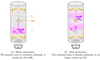 |
Fig. 1 Wave contained in a volume dV before and after interaction with the SRR in a waveguide. According to the law of conservation of angular momentum, the AM carried by the incident wave dℳi has been transferred to the SRR, exerting a torque Γ for a time dt. Dashed arrows indicate wave propagation direction. 1, 2, A and B: matched antennas; SS: Spider Silk; C: Camera. |
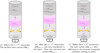 |
Fig. 2 AM transfer for the k + 1th interaction of a wave with the object. Dashed arrows indicate wave propagation direction. A’ and B’: antennas; C: Camera. |
Comparison of experimental results of spinning an SRR in a non-resonant waveguide and a non-resonant ring in a resonant waveguide, normalized by power.
2.3 Modeling for multiple interactions
We now examine how AM is transferred when the wave interacts several times with the object.
The first step is to model the interactions. The principle is illustrated in Figure 2. In the case studied, our cylindrical guide was transformed into a resonant cavity, short-circuited at both ends and fed by two antennas A’ et B’.
To begin with, we analyse what happens when a wave interacts once with an object. For this purpose, we consider an incident wave, in a volume dV, before its k + 1th interaction with the object. It carries an AM, denoted dℳi,k. This wave interacts with the object, transferring a proportion pt of the wave’s AM to the object. The object thus acquires a quantity of AM dℳobj,k+1 such that:
 (4a)
(4a)
Considering AM conservation, the wave scattered by the object carries an AM of dℳs,k+1 where:
 (4b)
(4b)
To continue, we look at what happens to the scattered wave. Part of the wave will be absorbed (and therefore lost) by antennas A’ and B’. It will then mostly reflected off the surfaces at the extremities of our resonant cavity, which are metallic electrical conductors. As a result, the direction of wave rotation does not change during reflection. The wave’s AM is therefore preserved, given some losses. Finally, part of the wave is lost again as it is absorbed by the antennas. This completes the cycle. Throughout this cycle, losses also occur through the lateral surfaces. It can be pointed out that the loss of energy is proportionally associated with a reduction in AM. More precisely, losses result in a transfer of AM to the lossy object. So, in our model, it’s not necessary to consider object losses, as they can already be included in pt. We denote pl the proportion of all the losses of AM due to the waveguide (including antennas, bottom, top and side surfaces). They result in a reduction in the AM of the wave by a transfer of dℳloss,k+1 to the waveguide:
 (4c)
(4c)
After reflecting off the surfaces at the extremities, the wave returns to the object, for its k + 2th interaction, with an AM dMi,k+1 verifying:
 (4d)
(4d)
This gives us:
 (4e)
(4e)
To complete our model, it should be pointed out that, in our experimental set-up, we use a continuous-wave power supply. Thus, in the volume dV under consideration, there is a overlapping wave components just emitted by the source, those that have already interacted once, those in their third interaction, etc. We denote N the number of interactions the wave can have with the object (theoretically, N → ∞). As a result, the total AM dℳi,tot,N of the incident wave in volume dV after N interactions is such that:
 (5a)
(5a)
The AM dℳobj,tot,N transferred to the object therefore and the lost AM (transferred to the guide) becomes:
 (5b)
(5b)
 (5c)
(5c)
It should be noticed that our model ensures the conservation of the AM, since the initially supplied AM dℳi,0 is distributed between the object (dℳobj,tot,N), the guide (dℳloss,tot,N) and the remaining AM in wave (dℳi,N), after the Nth interaction, such that:
 (5d)
(5d)
3 Results
The model we have developed enables us to identify the influence of the various AM transfers, and thereby, to move towards an optimum transfer, in the next steps. First, let’s examine the influence of each parameter in general, and then illustrate two important cases with numerical and experimental results.
3.1 Theoretical modeling results
Let’s analyze the results of this model. Note that the model of Equation (5) is, at least, valid for 0 ⩽ pt ⩽ 2 and 0 ⩽ pl ⩽ 2, as long as both |1 − pt| ≠ 1 and |1 − pl| ≠ 1.
The significance of cases 0 < pt < 1 and 0 < pl < 1 is obvious and will not be detailed here. However, by analogy with linear momentum, where the reflection of a wave on a PEC leads to the transfer of two times the momentum, an object can absorb, in one interaction, up to two times the AM of a wave. This happens when the scattered wave has an AM opposite to that of the incident wave, in other words, when the circular polarization changes direction. Thus, if 1 < pt ⩽ 2 or 1 < pl ⩽ 2, negative AM can then be obtained, reflecting a circular polarization rotating in the opposite direction.
Specific cases appear. The case pl = 0 is obviously not interesting since no AM transfer to the object takes place. The case pt = 0 means no loss in the waveguide. The case of pt = 1, all the AM of the wave is transferred to the object from the very first interaction. Consequently, subsequent interactions no longer generate AM transfers: these interactions are useless from an electrodynamic point of view. The pl = 1 case means that all the AM is ultimately transmitted to the guide: at most one interaction is possible. Note that this is the value we’re looking for the SRR in the waveguide as it will be discussed later.
The very special case of both pt = 2 and pl = 2, which appear of special interest and will be discussed in the discussion section.
Apart from these special cases, since |1 − pt| < 1 and |1 − pl| < 1, then it is theoretically possible to accumulate the transfer of an innite number of interactions (N → ∞).
Each new transfer is weaker than the previous one, but remains non-zero. Consequently, even if the transfer for an interaction is not optimal (pt << 1), it is still possible to accumulate the transfers and thus to improve the total AM transfer (and therefore the torque applied by the wave to the object). It is then straightforward to define the AM transfer efficiency ηobj from the wave to the experimental device, by:
 (6)
(6)
It can be immediately concluded from Equation (6) that, as soon as (1 − pt) and (1 − pl) are of the same sign, there is an interest in exploiting multiple interactions, given that ηobj > pt. Thus it appears that if pt > 1 (more than once the AM of the incident wave is transmitted to the object in one interaction) but pl < 1 (no change in the wave’s direction of rotation when it interacts with the waveguide), the multiple interactions are not useful since they interact destructively. In order to obtain ηobj > 1 (more than once the initial AM of the wave transferred to the object), it is necessary that pt > 1. To reach ηobj > 2 (more than twice the initial AM of the wave transmitted to the object), it can be shown that it requires both  and
and  . This will be detailed in the Discussion session.
3.2 Numerical and experimental illustrations of the use of resonances to improve AM transfer from wave to object
Let’s now illustrate this model and these analytical results with numerical and experimental examples. To do so, the same experimental set-up as in [1,2] is used. It is briefly described in Section 2.2.
3.2.1 Notes on the experimental set-up
As this setup is not perfect, let’s discuss the initial AM and the resulting torque that can be obtained consequently. Let ΦSAM,0 be the initial SAM flow and ΦSAM,obj the total SAM flow transferred to the object, such that:
 (7a)
(7a)
 (7b)
(7b)
For an elliptically polarized wave, Equation (1) can be modified as follows [10]:
 (8a)
(8a)
In Equation (8a), P is the power of the elliptically polarized wave, f is its frequency and φ indicates the ellipticity of the wave:
 (8b)
(8b)
Let Γth be the theoretical torque corresponding to the SAM transfer of the initial SAM flow, is then:
 (9a)
(9a)
 (9b)
(9b)
As a result:
 (9c)
(9c)
The wave generated by our experimental device is slightly elliptically polarized, and it can be found that sin(2ϕ) ≈ 0.82. See supplementary materials for further details. Losses between the generator and ports A and B can be estimated around 1dB i.e. power actually injected: P ≈ 0.80Pgenerator.
Thus, theoretical torque Γth, relative to the power Pgenerator supplied by the generator, values:
 (10)
(10)
Note that this is a purely indicative value. The underlying assumptions are strong (homogeneous field, incident elliptical polarization unmodified by the presence of the object, friction and restoring torque neglected, etc.).
3.2.2 SRR in a waveguide: illustration of a resonant object to improve an AM transfer in a single interaction
The results obtained in [1] can be used to illustrate the model developed in this article. In this configuration, a resonant object (the SRR) is suspended in a non-resonant waveguide (of inner diameter ϕint = 84 mm and a total length between antennas 1,2 and A,B of around 1.5λg that is ≈344 mm), as illustrated in Figure 3 and detailed in the supplementary materials.
It can be considered that the entire incident wave is absorbed by the waveguide antennas after interaction with the SRR (see the waveguide S parameters in the supplementary materials). In our model, this means that pl,waveguide = 1 and that there is therefore only one interaction. As a result:
 (11a)
(11a)
The protocol is described in [1] and only summarized here. The resonant frequency fres is empirically chosen to obtain maximum torque. Several supply powers are tested, and several measurements are made for each power. In each case, both directions of wave rotation are investigated. This ensures that the wave is the source of the movement. Using the camera, we measure the angular position of the dipole along the Δ axis. We consider only its first turn to limit the influence of unwanted phenomena (such as air friction or the wire’s restoring torque). This position is interpolated to determine the time average angular acceleration 〈αΔ〉 of the SRR around its axis. This enables us to calculate the time average torque 〈ΓΔ〉 exerted on the SRR, given that 〈ΓΔ〉 = JΔ〈αΔ〉. As explained later, since it was also shown in [1] that torque is proportional to power, we normalize the results by power. Experimentally, for a resonance frequency of 2.47GHz, an acceleration of 2.3.10−4 rev.s−2.W−1 is measured, corresponding to a torque of 1.8.10−2 nN.m.W−1. The experimental transfer efficiency is then ηSRR · · waveguide ≈ pt,SRR · · waveguide ≈ 41%.
Experimental results are summarized in Table 1 and model parameters derived from them in Table 2.
To investigate the role of resonance, we compare the SRR with a similar but non-resonant object. It was thus decided to suspend a simple copper ring, as a non-resonant magnetic dipole, instead of the SRR. It is similar to the SRR (in particular, it has the same dimensions and therefore almost the same rotational inertia JΔ), except that it has no gap. From a force perspective, the behavior is the same as for the SRR (see previous letter [1] for details). But since the ring is not resonant, the induced current is lower, and so is the resulting torque. In our AM model, it leads to a lower pt than that of the SRR. Using the same experimental protocol as above, no significant movement was experimentally detected. This confirms that its pt is extremely low. Using the same numerical model as in [1] (replacing the SRR with the copper ring and adding the experimental losses between the generator and the guide), we measure a torque of the order of 1.7.10−5 nN.m.W−1. This implies ηRing · · waveguide ≈ pt,Ring · · waveguide ≈ 0.04% ⪡ pt,SRR · · waveguide. This proves the value of SRR resonance.
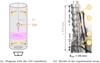 |
Fig. 3 Illustration of our experimental setup in waveguide: an SRR is suspended from a spider wire in a closed cylindrical waveguide, fed by antennas. Dashed arrows indicate wave propagation direction. 1, 2, A and B: matched antennas; SS: Spider Silk; C: camera. |
3.3 Copper ring in an electromagnetic cavity: illustration of the benefits of multiple interactions
To obtain multiple interactions, we seek to exploit a resonant electromagnetic cavity. To do so, we transform the experimental setup detailed in the previous letter [1]. Its configuration has been changed to remove antennas 1 and 2, adjust its length (around 599 mm) and the position of the antennas (about 122 mm from the lower extremity), in order to transform the guide into an electromagnetic resonant cavity. Figure 4 provides illustrations of the configuration adopted. Supplementary materials provide details of the configuration and the experimental S parameters. The same copper ring as described above is used as a non-resonant object. The same protocol is applied. For practical reasons, power levels differ due to practical constraints in the previous case, that is why the results are normalized by the power. Experimentally, the resonance frequency in cavity configuration is determined at 2.4356 GHz (see cavity S parameters in the supplementary materials). It is at this frequency that the fastest angular accelerations have been measured, with an acceleration of 1.3.10−4 rev.s−2 .W−1. It corresponds to a torque of 9.6.10−3 nN.mW−1. The experimental AM transfer efficiency is then ηRing · · cavity ≈ 22%. Assuming that pt,Ring · · cavity = pt,Ring · · waveguide, then we can estimate from Equation (6) that pl,cavity ≈ 0.001. Experimental results are summarized in Table 1 and model parameters derived from them in Table 2.
It should be emphasized that ηRing · · cavity ≈ 22% >> ηRing · waveguide ≈ 0.04%. The gain of putting in resonant cavity is unequivocal. The AM transfer efficiency of the ring in the resonant cavity remains lower than that of the SRR in the waveguide. This shows the value of exploiting a resonant object as done in [1].
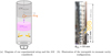 |
Fig. 4 Illustration of our experimental setup: a copper ring suspended from a spider wire in a closed cylindrical guide, fed by antennas, to constitute an electromagnetic resonant cavity. A’ and B’: antennas; SS: Spider Silk; C: Camera. |
Comparison of model parameters derived from numerical (★) and/or experimental (◇) measurements.
4 Discussion
The previous experimental studies prove the benefits of using resonances to efficiently transmit the AM of the incident wave to the object. Object resonance (illustrated by the case of SRR in waveguide configuration) seems to be the best transfer method. However, for a non-resonant object, the use of a resonant cavity has shown its usefulness. However, all these results show that less than once the incident momentum has been transferred to the object.
As shown by Equation (6) (see Sect. 3.1), in order to exceed the transfer of two times the momentum (ηobj > 2), it is necessary to have pt > 1. This requires at least a resonant object (with a stronger resonance than the SRR used here), correctly positioned in a resonant environment (at a distance  from one of the end walls of the cavity, for example). This implies exploiting several resonances, which can be experimentally difficult. Moreover, pt > 1 means that wave’s direction of rotation changes when it interacts with the object. To be able to accumulate several interactions constructively, this also implies that pl > 1. In the contrary case, after an interaction n with the object, the wave returns in the opposite direction of rotation (i.e. with an AM of opposite sign), giving rise to an effect at interaction n+1 that is the opposite of interaction n.
The optimal configuration is to get close to both pt = 2 and pl = 2. In this case, efficiency diverges to +∞. Figure 5 illustrates this case. As an example, for pt = 1.9 and pl = 1.9, one obtains ηobj ≈ 10. If pt = 1.99 and pt = 1.99, then ηobj ≈ 100.
As seen in Figure 5, this configuration raises an additional difficulty: How to generate an excitation that produces the desired configuration of the electromagnetic field (i.e. two opposite directions of rotation depending on the direction of propagation)?
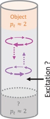 |
Fig. 5 Resonant cavity principle from an electrodynamic point of view: two different polarizations depending on propagation direction. The dotted arrows indicate the desired direction of propagation for each polarization. |
5 Conclusion
In conclusion, our aim is to spin objects with microwaves. Because the AM carried by a wave at these frequencies is weak, we seek to increase the AM transfer between the wave and the object. The way we propose is to make appropriate use of the resonance phenomenon. A first step was to exploit the resonance of an object, the SRR [1]. A second step was to test other resonant dipoles, such as resonant electric dipole [2]. This article represents the third step. It consists of trying to accumulate the effects of several interactions.
A simple model has been developed for this purpose. It shows that accumulation is possible. Under classical conditions (where at most once the AM of the wave can be transferred in one interaction), this accumulation is limited. At most one time the initial AM is finally transferred to the object. However, this can result in substantial total transfer to objects with a low ability to AM to be transferred. Numerical and experimental realizations illustrate this model. In addition to spinning a resonant object (SRR) in a non-resonant waveguide, as in [1], a non-resonant object in a resonant cavity has been experimentally investigated, in order to accumulate several interactions. The experimental setup previously used was converted into a resonant electromagnetic cavity. This resonant setup enabled us to spin a ring, reaching several revolutions in a few seconds, whereas conventional waveguide didn’t allow any rotation. The next step is to intelligently combine object resonance and cavity resonance. As shown by our model, even with pt > 1, in the resonant waveguide as it is, the maximum asymptotic transfer is limited to one unit of the wave’s initial AM. So it’s necessary to modify our resonant electromagnetic cavity, in order to convert it into a resonant electrodynamic cavity. We could then achieve a gain of several decades in object movement using microwaves.
Funding
The authors would like to thank DGA/AID and the company Any waves for co-funding this work.
Conflicts of interest
The authors have no conflicts to disclose.
Data availability statement
The data that support the findings of this study are available from the corresponding author upon reasonable request.
Author contribution statement
Côme Jodet: Conceptualization (equal); Investigation (lead); Methodology (equal); Software (lead); Validation (equal); Visualization (lead); Writing − original draft (lead); Writing − review & editing (equal). Olivier Pascal: Conceptualization (equal); Funding acquisition (equal); Methodology (equal); Resources (equal); Supervision (equal); Validation (equal); Writing − review & editing (equal). Jérôme Sokoloff: Conceptualization (equal); Funding acquisition (equal); Methodology (equal); Resources (equal); Supervision (equal); Validation (equal); Writing − review & editing (equal).
Supplementary Material
See supplementary materials for details of our experimental setups (waveguide and resonant electromagnetic cavity) and demonstrative videos of ring rotation in both polarization directions in the resonant electromagnetic cavity. Access Supplementary Material
References
- C. Jodet, O. Pascal, J. Sokoloff, Spinning a split ring resonator with microwaves, Appl. Phys. Lett. 123, 181103 (2023). https://doi.org/10.1063/5.0174364 [CrossRef] [Google Scholar]
- C. Jodet, O. Pascal, J. Sokoloff, Comparison of spinning centimetric resonant electric and magnetic dipoles with microwaves, in 2024 IEEE INC-USNC-URSI Radio Science Meeting (Joint with AP-S Symposium) (2024), pp. 26–27. https://doi.org/10.23919/INC-USNC-URSI61303.2024.10632318 [Google Scholar]
- J. Kepler, De cometis libelli tres, Typis Andreæ Apergeri, sumptibus Sebastiani Mylii bibliopolæ Augustani (1619) [Online]. Available: https://archive.org/details/den-kbd-pil-130011021221-001 [Google Scholar]
- J.C. Maxwell, A treatise on electricity and magnetism, Vol. 1 (Oxford: Clarendon Press, 1873) [Google Scholar]
- L. Page, A century’s progress in physics, Am. J. Sci. s4-46, 316 (1918). https://doi.org/10.2475/ajs.s4-46.271.303 [Google Scholar]
- O. Emile, J. Emile, Energy, linear momentum, and angular momentum of light: What do we measure?, Ann. Phys. (Berl.) 530, 1800111 (2018). https://doi.org/10.1002/andp.201800111 [CrossRef] [Google Scholar]
- R.A. Beth, Direct detection of the angular momentum of light, Phys. Rev. 48, 471 (1935). https://doi.org/10.1103/PhysRev.48.471 [CrossRef] [Google Scholar]
- R.A. Beth, Mechanical detection and measurement of the angular momentum of light, Phys. Rev. 50, 115 (1936). https://doi.org/10.1103/PhysRev.50.115 [NASA ADS] [CrossRef] [Google Scholar]
- A.H.S. Holbourn, Angular momentum of circularly polarised light, Nature 137, 31 (1936). https://doi.org/10.1038/137031a0 [CrossRef] [Google Scholar]
- N. Carrara, Torque and angular momentum of centimetre electromagnetic waves, Nature 164, 882 (1949). https://doi.org/10.1038/164882c0 [CrossRef] [PubMed] [Google Scholar]
- P.J. Allen, A radiation torque experiment, Am. J. Phys. 34, 1185 (1966). https://doi.org/10.1119/1.1972585 [CrossRef] [Google Scholar]
- M. Kristensen, M.W. Beijersbergen, J.P. Woerdman, Angular momentum and spin-orbit coupling for microwave photons, Opt. Commun. 104, 229 (1994). https://doi.org/10.1016/0030-4018(94)90547-9 [CrossRef] [Google Scholar]
- O. Sydoruk, E. Tatartschuk, E. Shamonina, L. Solymar, Analytical formulation for the resonant frequency of split rings, J. Appl. Phys. 105, 014903 (2009). https://doi.org/10.1063/1.3056052 [CrossRef] [Google Scholar]
Cite this article as: Côme Jodet, Olivier Pascal, Jérôme Sokoloff, How to optimize the extraction of the spin angular momentum of an electromagnetic wave using resonances, Eur. Phys. J. Appl. Phys. 100, 15 (2025), https://doi.org/10.1051/epjap/2025013
All Tables
Comparison of experimental results of spinning an SRR in a non-resonant waveguide and a non-resonant ring in a resonant waveguide, normalized by power.
Comparison of model parameters derived from numerical (★) and/or experimental (◇) measurements.
All Figures
|
Fig. 1 Wave contained in a volume dV before and after interaction with the SRR in a waveguide. According to the law of conservation of angular momentum, the AM carried by the incident wave dℳi has been transferred to the SRR, exerting a torque Γ for a time dt. Dashed arrows indicate wave propagation direction. 1, 2, A and B: matched antennas; SS: Spider Silk; C: Camera. |
| In the text | |
|
Fig. 2 AM transfer for the k + 1th interaction of a wave with the object. Dashed arrows indicate wave propagation direction. A’ and B’: antennas; C: Camera. |
| In the text | |
|
Fig. 3 Illustration of our experimental setup in waveguide: an SRR is suspended from a spider wire in a closed cylindrical waveguide, fed by antennas. Dashed arrows indicate wave propagation direction. 1, 2, A and B: matched antennas; SS: Spider Silk; C: camera. |
| In the text | |
|
Fig. 4 Illustration of our experimental setup: a copper ring suspended from a spider wire in a closed cylindrical guide, fed by antennas, to constitute an electromagnetic resonant cavity. A’ and B’: antennas; SS: Spider Silk; C: Camera. |
| In the text | |
|
Fig. 5 Resonant cavity principle from an electrodynamic point of view: two different polarizations depending on propagation direction. The dotted arrows indicate the desired direction of propagation for each polarization. |
| In the text | |
Current usage metrics show cumulative count of Article Views (full-text article views including HTML views, PDF and ePub downloads, according to the available data) and Abstracts Views on Vision4Press platform.
Data correspond to usage on the plateform after 2015. The current usage metrics is available 48-96 hours after online publication and is updated daily on week days.
Initial download of the metrics may take a while.