| Issue |
Eur. Phys. J. Appl. Phys.
Volume 93, Number 3, March 2021
International Symposium on Electromagnetic Fields in Mechatronics, Electrical and Electronic Engineering (ISEF 2019)
|
|
|---|---|---|
| Article Number | 30901 | |
| Number of page(s) | 7 | |
| Section | Physics of Energy Transfer, Conversion and Storage | |
| DOI | https://doi.org/10.1051/epjap/2020200027 | |
| Published online | 17 March 2021 | |
https://doi.org/10.1051/epjap/2020200027
Regular Article
Design of a superconducting machine and its cooling system for an aeronautics application★
University of Lorraine, GREEN, Nancy, France
* e-mail: This email address is being protected from spambots. You need JavaScript enabled to view it.
Received:
31
January
2020
Received in final form:
21
April
2020
Accepted:
16
November
2020
Published online: 17 March 2021
Abstract
The transition to electric propulsion aircraft requires electrical motors or generators with high power density. The “zero resistivity” of the superconducting materials could be used in electrical machines to produce high magnetic fields and reduce the use of heavy components such as the ferromagnetic parts. The discovery and recent developments in High Temperature Superconductors (HTS) technology make the superconducting machine a serious candidate in the future of aircraft. The design of a superconducting machine is strongly dependent on its electromagnetic and thermal behavior. In this paper, the design of a 50 kW superconducting aircraft generator is presented. The mass of the cryogenic cooling system is included into the design in order to optimize the entire superconducting system. The study shows that the choice of the cooling temperature to reduce the mass of the superconducting machine and its cooling system will depends on the input power of the machine.
Contribution to the Topical Issue “International Symposium on Electromagnetic Fields in Mechatronics, Electrical and Electronic Engineering (ISEF 2019)”, edited by Adel Razek.
© A. Colle et al., published by EDP Sciences, 2021
 This is an Open Access article distributed under the terms of the Creative Commons Attribution License (https://creativecommons.org/licenses/by/4.0), which permits unrestricted use, distribution, and reproduction in any medium, provided the original work is properly cited.
1 Introduction
The aerospace industry is primarily concerned by the move towards electric propulsion alternatives with the desire to improve fuel economy, reduced emissions or noises. The Boeing 787 Dreamliner is a concrete expression of this dynamic. The traditional pneumatic system was replaced by an electric one. The installed electric power reaches the MW level and is used to supply systems such as hydraulics, engines start or wing ice protections. However, almost all aircraft energy (∼90%) is dedicated to the propulsion, thus the major gain of efficiency should come from the propulsion system. The technology to propel electrically a large commercial aircraft is not yet ready but different projects, such as Solar Impulse or Airbus E-Fan, are advancing the technology. To supplant current propulsion technologies, the electrical machine masses must be reduced. The power-to-mass ratio is the main machine design indicator in this type of application.
In this context, some studies about superconducting machines have been conducted [1–3]. To date, there are few superconducting machines built with a power greater than MW and dedicated to aeronautic applications. Most of the major achievements have concerned naval propulsions or wind generators. These applications require low rotational speeds and therefore the specific powers are not important, unlike the specific torques. However, there are two examples [4,5] of SC machines for aeronautics application constructed, with specific power above 9 kW/kg. Superconductivity is a particular state of matter that exhibits zero electrical resistivity when cooled below a particular temperature called critical temperature. The value of this temperature depends on the material used. This feature allows a large electric current to flow through the superconducting material. The magnetic field in the air gap and the torque of an electrical machine using these materials can thus be increased. The magnetic field is one of the factors limiting the superconductor's operating current. However, this maximal current can be improved if the temperature of cooling is decreased. The problem is that the superconductors known have a critical temperature in the cryogenic domain, typically < ‑200 °C. So the use of these materials therefore requires a cooling system that becomes heavier and less efficient as the cooling temperature decreases. There is therefore a different behavior of the electrical machines and the cooling systems as a function of the cooling temperature. This leads us to believe that for each superconducting system, machine and cooling system, there exists an optimal temperature that reduces the total mass.
Beyond the large possibilities of superconducting machine topology [6,7], the flux modulation machine is selected because of its brushless structure. This electrical machine was already built in its radial form using low temperature superconductors [8,9]. For this project, the axial topology is selected which seems to have a higher power-to-mass ratio. The active components of this machine appear in Figure 1. Moreover, the electrical machine will use High Temperature Superconducting (HTS) materials which have a more flexible variation of cooling temperature than the low temperature one. The principle of operation and the components of this particular superconducting machine are explained in the first part of the paper. Then the second part is dedicated on the sizing of the superconducting system which include the superconducting machine and its cooling system. We will see that this study requires the knowledge of the electromagnetic and thermal behavior for which different semi-analytical, analytical and numerical models will be proposed.
 |
Fig. 1 View containing the active elements of the superconducting machine. |
2 The superconducting machine
As explained previously the superconductivity phenomenon appears under a critical temperature, depending on the material used. For the superconductors of this project, the temperature is 90 K for the YBCO and 110 K for the BSCCO. The study of the superconducting system is limited by data obtained from the manufacturer of superconducting materials. In our case, the different temperature tested will comprised between 77 K and 20 K.
The flux modulation machine is classified beyond the partially superconducting. The inductor is the only superconducting part and is composed by:
-
a HTS coil, which is supplied by a DC current and generates an axial magnetic field, called the main field.
-
several HTS pellets or shield, which reacts to the field of the HTS coil.
In the initial state, the superconducting elements are cooled below their critical temperature and no current is applied in the superconducting coil. Therefore, the total magnetic field is zero. Then, a ramp of current supplied the HTS coil. The HTS pellets see a variation of the flux so a current is induced by the Lenz law in order to oppose the main field. These currents, induced in the HTS pellets, will create a magnetic field that will oppose in direction the one created by the superconducting coil. So, the total magnetic field will be reduced near the pellets. Between two pellets, there is a non-magnetic and non-conducting material that has no effect on the magnetic field produced by the SC coil. So, if we consider Figure 1, the magnetic field is reduced behind an HTS pellet and equal to the magnetizing field between them. The combination of the coil and the SC pellets creates the spatial variation of the magnetic field necessary for any electrical machine. This superconducting phenomenon is called the diamagnetic response. Because of the zero resistivity of the superconductors, the current induced inside the HTS pellets are trapped and remains constant even once there no more variation of the magnetic flux density when the maximum DC current into is reached.
Finally, the remaining part of the machine is the armature winding which is composed by a three-phase copper winding. A concentric winding is used in our application in order to reduce the total weight. The real advantage of using superconductivity is to remove most of the ferromagnetic materials. Therefore, the iron teeth are removed while the thickness of the back-iron is largely reduced. Without iron teeth, more space can be dedicated to the copper coil in order to increase the electromagnetic torque.
Figure 2 shows the magnetic flux distribution on one copper coil of the armature winding. In Figure 2a, one part of the armature coil is exposed to a high magnetic field and the other part is shielded by the HTS pellet. This difference will create an electromagnetic torque. In Figure 2b, otherwise both part of the armature coil is submitted to the same level of magnetic field. As the current direction in these parts is opposite, the total electromagnetic force is zero. The main geometrical and electrical parameters of the superconducting machine are given in Table 1.
 |
Fig. 2 Magnetic behavior of the flux modulation machine in the (a) maximum torque configuration (b) minimum torque configuration. |
Electrical and geometrical parameters used for the superconducting machine.
3 Design of the superconducting machine
The superconducting machine design is based on the knowledge of the electromagnetic field and thermal behavior.
3.1 Electromagnetic design
The flux modulation, evoked previously, is a 3-D electromagnetic problem due to the intrinsic geometry of an axial-flux machine. This kind of numerical problem can be time consuming when dealing with the superconducting behavior [10]. Numerical methods, as Finite Element [11] or other methods described in [12], are however essential to calculate accurately the induced current inside the pellets and so the magnetic behavior of the superconducting inductor. For these methods, the variation in the resistivity of superconductors is given by a power law. This law depends on the material and is obtained from experimental measurements. In numerical models, the resistivity ρ of superconducting materials is written with: (1)
(1)
where E and J are respectively the electric field and the current density in the superconducting tape. Ec and Jc are the so-called critical quantities of superconducting materials. The standard sets Ec
at 1 μV/cm for high temperature superconductors. The maximum current density Jc
that can flow through the superconducting tape is reached when measuring E = Ec
. The parameter n represents how sharp is the change of the resistivity. In our problem, the temperature is an input, which is therefore imposed. The variation of Jc
and n with the magnetic field are obtained experimentally and then interpolated by [13]: (2)
(2)
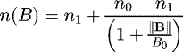 (3)where Jc0 is Jc
for ||B|| = 0, n1 and n0 are respectively the n-value for ||B|| = 0 and ||B|| ≫ B0 and B0, is the interpolation constant.
(3)where Jc0 is Jc
for ||B|| = 0, n1 and n0 are respectively the n-value for ||B|| = 0 and ||B|| ≫ B0 and B0, is the interpolation constant.
We will simplify the 3D problem of the machine into a 2D axisymmetric, shown in Figure 3a, in order to show how the current induced in the pellet is distributed. The parameters used for this simulation is described in Table 2. The HTS shield is placed into a magnetic flux density with a maximum value of 1.1 T. This magnetic field is equivalent to the one generated by the HTS coil at the mean radius. Figure 2a represents the 2D axisymmetric problem solved using the relation (1).
The 2D distribution of the current density is shown in Figure 3b. This distribution is typical of superconductors, there is an area where the current density is equal to its critical value, i.e. ≈1000 A/mm2 and an area where the current is zero. The results are shown in the superconducting pellet's heart in Figure 4. The penetration length of the current Lp is calculated on the axis of symmetry of the superconducting pellet according to the thickness. Then, the distance where the current is different of 0 correspond to Lp. The value of the penetration for the 2D axisymmetric model is 2 mm, or 5% of the HTS shield. As expected, beyond this region where the superconducting current is zero, the magnetic induction is perfectly vanished by the screen's diamagnetic reaction. The magnetic flux density is also plotted 5 mm above the HTS pellet in order to observe the flux modulation principle.
The use of the non-linear resistivity law makes the resolution of the problem very time-consuming. The design process therefore consists in carrying out a sizing of the superconducting machine with a perfect diamagnetic behavior of the HTS shields. This hypothesis is correct only if the penetration depth is sufficiently small compared to the size of the pellet and decreases significantly the computation time. The magnetic distribution over a pole angle is calculated using the finite element method with the diamagnetic hypothesis and represented in Figure 5. In the same figure in dotted line, the flux modulation with the real behavior in 3D now, using (1), is shown. In this situation, the perfect diamagnetic behavior is good.
An example of the penetration length's effect on the torque is shown in Figure 6 with the superconducting machine described by Table 1. In this case, the torque is divided by 2 when the current penetrates 1/4 of the superconducting pellet. Once the sizing choices made, a numerical resolution using (1) should validate this design.
 |
Fig. 3 (a) 2D axismetric problem solved. (b) 2D distribution of the current density norm. |
Electrical and geometrical parameters used for the HTS shield simulation.
 |
Fig. 4 Magnetic flux density and current density penetration into the HTS shield. |
 |
Fig. 5 Magnetic distribution behind a HTS pellet at different radius. |
 |
Fig. 6 Decrease of the torque with Lp. |
3.2 Thermal design
3.2.1 Non-cryogenic region
The copper coils and back iron are considered in the thermal design. The losses in these elements occur in a thermal model that determines the maximum value of the current in the coils of the armature winding. The temperature of the copper wires should be investigated to not exceed the maximum temperature of the electric insulation.
These elements operate at ambient temperature. The DC losses of the non-superconducting elements are obtained by the classical methods.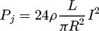 (4)where R is the radius of the wire, ρ the resistivity of the copper, L the total length of one coil and I the effective current flowing through the coil. The coefficient in (2) corresponds to the number of coils for a 12/10 winding with double stator topology.
However due to the absence of iron teeth, the magnetic field on the copper wire is important and contribute to generate large AC losses. A standard analytical formula is used. It gives the analytical solution of the eddy current losses in a single round conductor laying in sinusoidal magnetic field. (5)where l is the length of the conductor exposed to the AC magnetic field, f the frequency of the magnetic field and B is the effective value of the magnetic flux density seen by the conductor.
In order to obtain the total eddy current losses, the calculation must be performed on every conductor of each coil. The magnetic field in the air gap of an electrical machine is composed of several harmonics that also creates AC losses, the method described by Wang et al. is then used [15].
The iron losses PI
are composed of hysteresis losses Physt
, eddy current losses Pe
, and additional losses Padd
, which is an empirical corrective factor [16] (6)Most of the coefficients of (4) are empirical, however when the skin effect can be neglected the coefficient of eddy current losses for a lamination thickness d is:
 (7)
(7)
where ρ the resistivity of the copper
The coefficients of hysteresis losses and additional losses are generally obtained from the material manufacturer's curve. An iron with 3% of silicon was chosen for this application.
3.2.2 Cryogenic region
At cryogenic temperature, the AC losses in the superconducting pellets and the thermal losses are studied. The harmonics generated by the armature winding create the AC losses in the superconducting elements.
The thermal losses are estimated by the analytical equations for conduction and radiation losses. The convection losses are negligible because superconducting elements are placed in the vacuum. All equations for the calculation of cryogenic losses have been presented in a previous work [17].
3.3 Optimization of the superconducting system
The mass optimization of the superconducting system (superconducting machine and its cooling system) is then achieved by combining electromagnetic and thermal models. The detail of the optimization phase is shown in Figure 7. We will use a genetic algorithm (GA) in order to find a solution to this highly non-linear problem. The optimization algorithm is the GA implemented in MATLAB. Start with a given cooling temperature, the geometric variables, seen in Table 1, are randomly generated by the GA. The dimensions of the coil and the cooling temperature will size the Jc and thus the torque, the joule and iron losses as well as the mechanical stresses on the coil are obtained by a semi-analytical model [18]. The rest of the parameters are used for the thermal and mass calculation of the machine.
The mass of the superconducting machine Mmotor is calculated with the volume of every active and non-active element accounted for.
The cryogenic losses Pc
in the cryostat is correlated with the mass of the cooling system Mcooler
. The following relation gives a trend-line equation based on the current technology of cryocooler to link the mass, the losses and the operating temperature T [19]: (8)
(8)
Behind this equation is mainly hidden the weight of the cold-head, the compressor, the connection between the cold-head and the compressor, the cold-head cryostat. The optimization of a superconducting system is performed on two different machines. The first one uses the first generation of superconducting tape (BSCCO) and has a power of 50 kW, shown in Figure 8. The second is a 1 MW machine that uses the second generation of superconducting tape (YBCO), the results are presented in Figure 9.
As a result, the optimal temperature depends on the application. This result shows that a superconducting system is not optimal at low temperatures because the power/weight of the cooling system is too important for these temperatures. On the other hand, for a temperature close to the liquid nitrogen one, the performance of the superconductors becomes low and the power of the machine, constraint of the optimization, is achieved by increasing the volume/weight of the machine and the amount of superconducting material used. Concerning the machine of 50 kW, the highest power-to-mass ratio is obtained with an operating temperature of 66 K. While this temperature is 50 K for the 1 MW machine. At these temperatures, the power-to-mass ratio is 0.6 kW/kg for the 50 kW and 6 kW/kg for the 1 MW. High temperature superconductors are usually cooled at 30 K in superconducting machine application. However, if the mass of the superconducting system must be optimized, the whole system is 20% heavier at this temperature in the 1 MW case. The mass of the cooler doesn't increase a lot with the power (50 kg for 50 kW and 80 kg for 1 MW). This shows the interest for high power superconducting machine because the mass of the cooler increases slower than the mass of the machine.
Finally, Table 3 presents the evolution of the mass of the non-active elements of the superconducting machine using the YBCO technology. It can be seen that these masses, mainly due to the weight of the cryostats, do not evolve proportionally with the total mass of the machine. This result shows that a superconducting machine can be penalizing for a low power machines but interesting for higher powers.
 |
Fig. 7 Optimization process. |
 |
Fig. 8 Optimization of a superconducting machine of 50 kW with its cooling system. |
 |
Fig. 9 Optimization of a superconducting machine of 1 MW with its cooling system |
Evolution of the mass of the YBCO machine with the power.
4 Conclusion
The sizing of a superconducting system requires the knowledge of the magnetic and thermal behavior of the machine. The optimal operating temperature of a superconducting system depends on the power of the machine and the generation of superconducting tape used.
On the examples given, we observed that the superconducting technology is more interesting in terms of power-to-mass ratio than the standard technology of machine (about 5 kW/kg) for a MW-class machine [20].
These optimal temperatures are obtained with a trend-line on the current technology of cryocooler. These cooling systems are not specially designed for aircraft. So, in the future, the power-to-mass ratio is expected to increase with the development of new cryocooler.
Finally, a 50-kW prototype was built, based on this topology [21]. A presentation of the different step of manufacturing and the cooling system is presented in this work.
Author contribution statement
Alexandre COLLE developed the model to accurately and quickly design a superconducting system to reduce the total weight.
Thierry LUBIN & Jean LEVEQUE assisted the main author with their ideas and experience in the design of a superconducting machine.
Acknowledgments
The author would like to thank the Direction Générale de l'Armement (DGA) and Safran Tech for it support and interest.
References
- J.L.B. Felder, Turboelectric Distributed Propulsion in a Hybrid Wing Body Aircraft, presented at 20th International Society for Airbreathing Engines, Gothenburg, Sweden, 2011 [Google Scholar]
- C.A. Luongo et al., IEEE Trans. Appl. Supercond. 19 , 1055 (2009) [Google Scholar]
- K.S. Haran et al., Supercond. Sci. Technol. 30 , 123002 (2017) [CrossRef] [Google Scholar]
- R. Blaugher, in IEEE/CSC & ESAS European Superconductivity News Forum, No. 20 (2012), pp 4‑8 [Google Scholar]
- K. Sivasubramaniam et al., IEEE Trans. Appl. Supercond. 19 , 1656 (2009) [Google Scholar]
- P.N. Barnes, M.D. Sumption, G.L. Rhoads, Cryogenics 45 , 670‑686 (2005) [Google Scholar]
- J.R. Hull, M. Strasik, Supercond. Sci. Technol. 23 , 124005 (2010) [Google Scholar]
- E.H. Ailam, D. Netter, J. Leveque, B. Douine, P.J. Masson, A. Rezzoug, IEEE Trans. Appl. Supercond. 17 , 27 (2007) [Google Scholar]
- P. Masson, J. Leveque, D. Netter, A. Rezzoug, IEEE Trans. Appl. Supercond. 13 , 2239 (2003) [Google Scholar]
- K. Berger et al., IEEE Compumag (2017) [Google Scholar]
- B. Douine, G. Malé, T. Lubin, S. Mezani, J. Lévêque, K. Berger, J. Superconduct. Novel Magn. 27 , 903 (2014) [Google Scholar]
- F. Sirois, F. Grilli, Supercond. Sci. Technol. 28 , 043002 (2015) [Google Scholar]
- K. Berger, J. Lévêque, D. Netter, B. Douine, A. Rezzoug, IEEE Trans. Appl. Supercond. 17 , 3028 (2007) [Google Scholar]
- S. Zou, V.M. Zermeño, F. Grilli, IEEE Trans. Appl. Supercond. 26 , 1 (2016) [Google Scholar]
- R. Wang, A.J. Kamper, in Conference Record of the 2002 IEEE Industry Applications Conference. 37th IAS Annual Meeting (Cat. No.02CH37344) (2002), vol. 2, p. 1289‑1294 [Google Scholar]
- D. Kowal, P. Sergeant, L. Dupré, L. Vandenbossche, IEEE Trans. Magn. 51 , 1 (2015) [CrossRef] [PubMed] [Google Scholar]
- A. Colle, S. Ayat, T. Lubin, O. Gosselin, J. Leveque, Evaluation des Pertes dans une Machine Supraconductrice à Modulation de Flux , SGE symposium, 2018 [Google Scholar]
- A. Colle, T. Lubin, S. Ayat, O. Gosselin, J. Lévêque, IEEE Trans. Magn. 55 , 1 (2019) [Google Scholar]
- H.J.M. ter Brake, G.F.M. Wiegerinck, Cryogenics 42 , 705 (2002) [Google Scholar]
- X. Zhang, C.L. Bowman, T.C. O'Connell, K.S. Haran, IET Electr. Power Appl. 12 , 767 (2018) [Google Scholar]
- A. Colle, T. Lubin, S. Ayat, O. Gosselin, J. Lévêque, Construction of a Flux Modulation Superconducting Machine for Aircraft , ASC, 2018 [Google Scholar]
Cite this article as: Alexandre Colle, Thierry Lubin, Jean Leveque, Design of a superconducting machine and its cooling system for an aeronautics application, Eur. Phys. J. Appl. Phys. 93, 30901 (2021)
All Tables
All Figures
|
Fig. 1 View containing the active elements of the superconducting machine. |
| In the text | |
|
Fig. 2 Magnetic behavior of the flux modulation machine in the (a) maximum torque configuration (b) minimum torque configuration. |
| In the text | |
|
Fig. 3 (a) 2D axismetric problem solved. (b) 2D distribution of the current density norm. |
| In the text | |
|
Fig. 4 Magnetic flux density and current density penetration into the HTS shield. |
| In the text | |
|
Fig. 5 Magnetic distribution behind a HTS pellet at different radius. |
| In the text | |
|
Fig. 6 Decrease of the torque with Lp. |
| In the text | |
|
Fig. 7 Optimization process. |
| In the text | |
|
Fig. 8 Optimization of a superconducting machine of 50 kW with its cooling system. |
| In the text | |
|
Fig. 9 Optimization of a superconducting machine of 1 MW with its cooling system |
| In the text | |
Current usage metrics show cumulative count of Article Views (full-text article views including HTML views, PDF and ePub downloads, according to the available data) and Abstracts Views on Vision4Press platform.
Data correspond to usage on the plateform after 2015. The current usage metrics is available 48-96 hours after online publication and is updated daily on week days.
Initial download of the metrics may take a while.