© B. Kane et al., EDP Sciences, 2020

1 Introduction

Electromagnetic induction welding of carbon fiber composites with thermoplastic matrix is a very promising technology for aircraft and space industry over the coming years. Compared with existing processes, it requires less energy, and the cycle times are shortened which allows us to overcome some issues associated with classical assembly techniques [1].

Figure 1 shows a classic configuration of a structural part of the aircraft (fuselage). The skin (composite 2) is reinforced by omega (composite 1). The skin is the bottom plate; omega is the upper piece in shape of omega which strengthen the structure. To obtain a good assembly, it is necessary to heat the interface up to the melting point of the thermoplastic matrix (350 °C). To avoid material deconsolidation, the temperature of the remaining volume is kept below the target temperature. To achieve this objective, the induced electromagnetic power must be mainly located nearby the interface area.

Composite carbon fiber material is a piling up of unidirectional plies layered with different orientations (Fig. 2). In each ply, the electrical conductivity ratio between the conductivity along fiber direction and transverse direction is higher than σ_///σ_T > 10⁴. No flow of induced current loops in the same ply during the induction phenomenon, if not the induced power would be extremely low. Due to electrical percolation phenomena, a current path between plies is then established and could be different according to the ply sequence [2].

Induction heating ensures fast and contactless injection of electromagnetic power into composite materials and paves the way to new processes in technological breakthrough either for assembly (welding) or for the evaluation of material health (non-destructive testing) [2]. However, due to the overly complex nature of these materials, the absorption zone of the electromagnetic fields is still too diffuse. To have a better control of electromagnetic power location, we have three degrees of freedom: the orientation of the plies, the addition of an insert material at the interface, and/or the insulation between plies (i.e. to have a degree of freedom on the conductivity of the plies). To investigate these possibilities, modeling tools are required. A 3D multi-physical model is extremely relevant but is very time-consuming because many cases must be investigated. In this paper, an original approach based on a coupling between 1D and 3D models is presented. The first one helps investigate different families of possibilities to optimize the ply sequence and the location of the power to realize the desired functionality. A three-dimensional magneto-thermal modeling [3] is then used to optimize pre-selected configurations.

Fig. 1 Airframe welding configuration of two composite materials.

Fig. 2 1D system representation.

2 1D model description

This study involves the electromagnetic and thermal modeling of the system. Two models are thus released: the electromagnetic model that goes through the recall of Maxwell's equations and the behavior laws of materials and the thermal model that is defined by the heat diffusion equation.

For 1D modeling, the welding system in Figure 1 is reduced to a 1D system as shown in Figure 2. The layer colored in blue is the interface between the two composites. It represents the insert layer in the case of an insert addition.

2.1 Electromagnetic model

The magnetic field at a layer (fold or ply) k of the configuration is governed by equation (1) [4].$$\mathrm{c}\mathrm{u}\mathrm{r}\mathrm{l}((1/{\sigma }_k)\mathrm{c}\mathrm{u}\mathrm{r}\mathrm{l}(H_k))+2j\pi f{\mu }_k{H}_k=0$$(1)

with μ_k the magnetic permeability, σ_k the electrical conductivity of the layer k and f the frequency.

Since the source field H₀ is assumed to be tangential and the plies infinitely long, (1) admits a solution in the form in (2).$$H_k(z)=A_k\exp (-{\gamma }_k{z}_k)+B_k\exp ({\gamma }_k{z}_k)$$(2)

where γ_k = (1 + j)/δ_k with the skin depth ${\delta }_k=\sqrt{1/(\pi f{\sigma }_k{\mu }_k)}$.

The constants A_k and B_k of a layer k are calculated according to electromagnetic transition conditions between layers k + 1 and k ‑ 1. For example, between the layer k (1 < k < n) and the layer k + 1, we have the relations in (3).$$\{\begin{array}{l}{H}_k(z_k=+t_k/2)=H_{k+1}(z_{k+1}=-t_{k+1}/2)\hfill \\ E_k(z_k=+t_k/2)=+E_{k+1}(z_{k+1}=-t_{k+1}/2)\hfill \end{array}$$(3)

with E_k = ∂H_k/(σ_k ∂z_k) the electric field at a layer k.

At the borders of the system (layers 1 et n), we have the conditions in (4).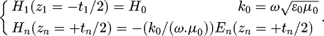$$\{\begin{array}{l}{H}_1(z_1=-t_1/2)=H_0{k}_0=\omega \sqrt{{\epsilon }_0{\mu }_0}\hfill \\ H_n(z_n=+t_n/2)=-(k_0/(\omega .{\mu }_0))E_n(z_n=+t_n/2)\hfill \end{array}.$$(4)

The resolution of (2) gives the value of the magnetic field H at any point z of the system. Starting from these values, we can deduce all the useful quantities such as the induced power density q and the induced current density J defined by equation (5).$$q(z)={\parallel J(z)\parallel }^2/\sigma \text{where}J(z)=\partial H(z)/\partial z$$(5)

2.2 Thermal model

The first principle of thermodynamics translates the energy conservation equation (Eq. (6)) which defines the thermal behavior of the material as a function of time tt [5].$$\mathrm{d}\mathrm{i}\mathrm{v}(\lambda \cdot \mathbf{g}\mathbf{r}\mathbf{a}\mathbf{d}(T))+q=\rho \cdot Cp\cdot \partial T/\partial tt$$(6)with ρ the specific mass, Cp the specific heat of the material, λ its thermal conductivity and T the temperature at the given point.

In this study, the temperature $T{(}_z^{tt})$ varies along a single axis z and the time tt, thus (6) becomes (7).$$\frac{\partial \lambda (z)}{\partial z}.\frac{\partial T\left(\begin{array}{l}tt\hfill \\ z\hfill \end{array}\right)}{\partial z}+\lambda (z).\frac{{\partial }^{2}T\left(\begin{array}{l}tt\hfill \\ z\hfill \end{array}\right)}{\partial z^2}+q(z)=\rho .Cp.\frac{\partial T\left(\begin{array}{l}tt\hfill \\ z\hfill \end{array}\right)}{\partial tt}$$(7)

This equation is solved by the finite difference method which considers all the non-linearities of physical properties. This resolution passes through the discretization of the layer thickness in Δz and the time in Δtt. Which allows us to write the relations in (8).$$\{\begin{array}{l}{\partial }^{2}T\left(\frac{\pi }{z}\right)/\partial z^2=\left(T\left(\frac{\pi }{z+\Delta z}\right)+T\left(\frac{\pi }{z-\Delta z}\right)-2T\left(\frac{\pi }{z}\right)\right)/{\left(\Delta z\right)}^2\hfill \\ \partial T\left(\frac{\pi }{z}\right)/\partial z=\left(T\left(\frac{\pi }{z}\right)-T\left(\frac{\pi }{z-\Delta z}\right)\right)/\left(\Delta z\right)\hfill \\ \partial T\left(\frac{\pi }{z}\right)/\partial tt=\left(T\left(\frac{\pi }{z}\right)-T\left(\frac{\pi -\Delta \pi }{z}\right)\right)/(\left(\Delta tt\right)\hfill \\ \partial \lambda (z)/\partial z=(\lambda (z)-\lambda (z-\Delta z))/(\Delta z)\hfill \end{array}$$(8)

To find solutions to this problem, it is necessary to set boundary conditions. In our case, the conditions are heat convection type defined in (9) and explained in [5]. h is the thermal convection coefficient (Wm⁻² K ⁻¹) and T_a the ambient temperature.$$[\lambda ].\partial T/\partial n=h(T-Ta)$$(9)

3 3D formulation

The phenomena related to electromagnetic induction welding are multi-physical and multi-scale. Moreover, the important scale factor between the macroscopic scale and the microscopic scale of composite materials could lead to important calculation cost. The 3D computational codes in A -ϕ formulation (Eq. (10)) developed in [2] are used for the electromagnetic simulation of our system.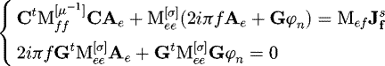$$\{\begin{array}{l}{\mathbf{C}}^t{\mathrm{M}}_{ff}^{[{\mu }^{-1}]}\mathbf{C}{\mathbf{A}}_e+{\mathrm{M}}_{ee}^{[\sigma ]}(2i\pi f{\mathbf{A}}_e+\mathbf{G}{\varphi }_n)={\mathrm{M}}_{ef}{\mathbf{J}}_{\mathbf{f}}^s\hfill \\ 2i\pi f{\mathbf{G}}^t{\mathrm{M}}_{ee}^{[\sigma ]}{\mathbf{A}}_e+{\mathbf{G}}^t{\mathrm{M}}_{ee}^{[\sigma ]}\mathbf{G}{\varphi }_n=0\hfill \end{array}$$(10)

where [σ] tensor is obtained with the help of homogenization techniques. C and G are the discrete counterparts of curl and grad operators, ${\mathbf{\text{A}}}_{\text{e}}={\sum }_{i=1}^E{w}^{e_i}{\mathbf{\text{A}}}_{\text{e}}^{\text{i}}$, ${\varphi }_n={\sum }_{i=1}^N{\omega }^{n_i}{\varphi }_n^i$ and ${\mathbf{\text{J}}}_{\mathbf{\text{f}}}^{\mathbf{\text{s}}}$ the circulations of the current source J^s calculated on the facets of the mesh. $M_{ff}^{[{\mu }^{-1}]}$, $M_{ee}^{[\sigma ]}$ and M_ef are mass matrices of the problem.

Equation (6) is used to solve the thermal problem in the composite plate with the Fourier boundary condition defined in (9). The heating problem is solved using a 3-D anisotropic finite-element method with different thermal conductivities along the fiber axis and transverse fiber axis.

To allow a reasonable comparison between 1D and 3D model, a U-shaped inductor, following Figure 3, is used to obtain a tangential field under the active part of the inductor.

Fig. 3 3D welding configuration.

4 Focusing of electromagnetic field

In this section, we study the impact of plies orientation, plies insulation, and addition of insert on the welding process. 1D model allows to pre-optimize the configuration. 3D model allows us to refine the results.

First, it is considered that the composites 1 and 2 consist of 15 unidirectional plies successively oriented at 0 and 90° ([0/90/0/90/0/90/0/90/0/90/0/90/0/90/0] or [[0/90]₇/0]). The idea here is to compare 1D and 3D models. A comparison between 1D and 3D models shows the same order of magnitude and physical behavior shown in Figure 4. We notice that all the power density is in the 0° plies. This power distribution prevents any welding between the two composites. To obtain a good welding, a ply sequence where the power is more localized nearby the interface is aimed.

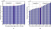Fig. 4 Distribution of electromagnetic power density for ${[{[0/90]}_7/0]}_s$. (a) 1D model. (b) 3D model.

4.1 Plies orientation

Our first investigation of the electromagnetic power focusing consists modifying the ply-sequence of the composite material. Because the 1D approach is extremely fast, all possible configurations could be investigated with an automatic process. As a result, a candidate that seems serious to us for a focus of power at the interface of the two composites is obtained. The ply sequence is the same for both composites and is ${[0_2/{45}_2/-{45}_2/{90}_2]}_s$. 0₂ means two adjacent layers oriented 0° from X-axis and subscript “s” means the next 8 plies has symmetric orientation from previous ones. Figure 5 shows its electromagnetic response with our one-dimensional tool.

Here, the power is brought to the interface between the two composites, but a large part of the power is also located at the outer ends of the composites.

With the 3D tool, the same configuration is simulated. The observation remains the same as illustrated in Figure 6. There is some difference between the power distributions with the 1D tool and those with the 3D model. Nevertheless, with the results of 1D we know what to expect from 3D.

This investigation track has its limits because the power located on the plies on the outer ends of the two composites is especially important. To overcome this problem, the modification of the local properties of the composites is investigated in the following section.

Fig. 5 Distribution of power density for ${[0_2/{45}_2/-{45}_2/{90}_2]}_s$ in 1D.

Fig. 6 Distribution of power density for ${[0_2/{45}_2/-{45}_2/{90}_2]}_s$ in 3D.

4.2 Insulation of the plies

The idea here is to insert thin layers of resin (with a thickness of 10 μm) between the plies located at the outer ends of the two composites. Figure 7 shows the electromagnetic power distribution obtained in this case.

We can notice that the resin layers have forced the induced currents to flow differently. In this way there was a clearer focus at the interface of the two composites.

Figure 8 shows the thermal response of this configuration. The temperature is well centered at the interface, but the welding width is very wide.

Fig. 7 Distribution of electromagnetic power with insulation of the plies.

Fig. 8 Temperature in the center of composites with insulation of the plies.

4.3 Addition of an insert

Our last investigation is to add a highly conductive layer with target properties between the two composites to be welded. The insert must be able to concentrate the heating power, thus permitting the welding of the two composites. The composites are like those in Figure 4. To find the right properties of the insert an optimization simulation was done with our 1D tool. The optimization variables, in this case, are the magnetic field H0, the electrical conductivity σ, the magnetic permeability µ of the insert, and the convection coefficients h1 and h2 respectively of the inductor side and the external side of the composite 2. Playing on the convection coefficients means that a cooling system can be added to each side of the plate composed to the two composites. A coefficient of 10 W/m²/K means that the corresponding side does not need a cooling system, so it can be left in the open air. NSGA-II, Non-dominated Sorting Genetic Algorithm II, is used for better robustness [6] to meet two contradictory objectives. On the first hand, it is necessary to have a temperature of 400 °C ± 10 in the insert layer (f1 = 1000* (T ‑ 400)²) and, on the other hand, to have a temperature that is as low as possible in the plies adjacent to the insert (f2 = exp(3* (T/100 ‑ 2)).

The realization of this optimization is done using MATLAB. After 5201 number of function calls and 103 generations, a Pareto front is generated where the different optimal combinations of the optimization variables are highlighted. In these series of combinations, the one that best meets our objectives is chosen (Tab. 1). By exploiting the data in [7], an insert with these target properties can be obtained with cobalt alloys.

With these optimized parameters of the insert, we simulate the configuration shown in Figure 2. All the electromagnetic power is located at the insert layer as shown in Figure 9. This is justified by the superior properties of this layer.

Figure 10 shows the temperature map according to thickness and time. At a heating time of 10 seconds, the temperature in the insert layer is 392 °C. This temperature is the highest in the studied system and does not exceed the material degradation limits (<400 °C). This is in the image of the power induced in this layer which represents 81% of the total power induced as shown in Figure 9.

To refine the results found, a simulation with the 3D tool developed was done. The current of the inductor is set to have the same magnetic field profile in the center of the plate as in the one-dimensional case (Fig. 3). The thermal response of this simulation is shown in Figure 11.

We can see that the curve obtained follows the same logic as that in 1D. The slight difference between the curves is mainly due to the shape of the inductor, the phenomena of edges, and the hypothesis made in 1D. Indeed, the magnetic field on the external phase of the composite 1 is assumed constant and tangential to it, which is not the case in 3D simulation. Nevertheless, a good concordance of the results is obtained.

Fig. 9 Distribution of power density for ${[{[0/90]}_7/0]}_s$ with an insert.

Fig. 10 Temperature in the center of composites with an insert in 1D.

Fig. 11 Temperature in the center of composites with an insert in 3D.

5 Conclusion

In this article, a 1D hybrid method (analytical for the electromagnetic part and digital for the thermal part) for solving electromagnetic induction heating problems was proposed. The different results allowed us to see the robustness and the speed (1.86s by iteration) of this method coupled to an optimization algorithm. This tool is very effective for predetermining the pair (σ, μ_r) of the insert, in particular for a very large number of plies. Nevertheless, the use of a 3D numerical simulation is necessary to refine the results and consider the inter-plies phenomena.

Author contribution statement

B. Kane has performed computation of the 1D model according to the original idea of D. Trichet. B. Kane has also adapted and performed the computation of the 3D model developed by G. Wasselynck and H. K. Bui. B. Kane wrote the manuscript with support from all co-authors. G. Wasselynck, G. Berthiau, and D. Trichet have conceived the original idea; G. Berthiau and D. Trichet have supervised the project. All authors have discussed the results and contributed to the final manuscript.

References

All Tables

All Figures

	Fig. 1 Airframe welding configuration of two composite materials.
In the text

	Fig. 2 1D system representation.
In the text

	Fig. 3 3D welding configuration.
In the text

	Fig. 4 Distribution of electromagnetic power density for ${[{[0/90]}_7/0]}_s$. (a) 1D model. (b) 3D model.
In the text

	Fig. 5 Distribution of power density for ${[0_2/{45}_2/-{45}_2/{90}_2]}_s$ in 1D.
In the text

	Fig. 6 Distribution of power density for ${[0_2/{45}_2/-{45}_2/{90}_2]}_s$ in 3D.
In the text

	Fig. 7 Distribution of electromagnetic power with insulation of the plies.
In the text

	Fig. 8 Temperature in the center of composites with insulation of the plies.
In the text

	Fig. 9 Distribution of power density for ${[{[0/90]}_7/0]}_s$ with an insert.
In the text

	Fig. 10 Temperature in the center of composites with an insert in 1D.
In the text

	Fig. 11 Temperature in the center of composites with an insert in 3D.
In the text

References

- R. Rudolf, P. Mitschang, M. Neitzel, Compos. Part A Appl. Sci. Manuf. 31, 1191 (2000) [Google Scholar]
- G. Wasselynck, D. Trichet, J. Fouladgar, IEEE Trans. Magn. 49, 1825 (2013) [Google Scholar]
- H.K. Bui, G. Wasselynck, D. Trichet, B. Ramdane, G. Berthiau, J. Fouladgar, IEEE Trans. Magn. 49, 1949 (2013) [Google Scholar]
- O. Bíró, Comput. Methods Appl. Mech. Eng. 169, 391 (1999) [Google Scholar]
- Y. Jaluria, K.E. Torrance, Computational Heat Transfer (Taylor & Francis, New York, 2003) [Google Scholar]
- K. Deb, Multi-objective optimization using evolutionary algorithms: an introduction, KanGAL Rep. Number 2011003, pp. 1–24, 2011 [Google Scholar]
- MatWeb, http://www.matweb.com [Google Scholar]
Cite this article as: Banda Kane, Guillaume Wasselynck, Huu Kien Bui, Didier Trichet, Gérard Berthiau, Focalization of electromagnetic power at the interface between two composites materials for induction welding, Eur. Phys. J. Appl. Phys. 91, 10902 (2020)