| Issue |
Eur. Phys. J. Appl. Phys.
Volume 89, Number 3, March 2020
|
|
|---|---|---|
| Article Number | 30701 | |
| Number of page(s) | 6 | |
| Section | Imaging, Microscopy and Spectroscopy | |
| DOI | https://doi.org/10.1051/epjap/2020200012 | |
| Published online | 12 May 2020 | |
https://doi.org/10.1051/epjap/2020200012
Regular Article
Stimulated Brillouin gain spectroscopy in a confined spatio-temporal domain (30 μm, 170 ns)
1
Laboratoire Kastler Brossel, ENS-PSL Université, Sorbonne Université, CNRS, Collège de France,
24 rue Lhomond,
75005
Paris,
France
2
Université d’Evry-Val d’Essonne, Université Paris-Saclay, Boulevard François Mitterrand,
91000
Evry,
France
* e-mail: This email address is being protected from spambots. You need JavaScript enabled to view it.
Received:
17
January
2020
Received in final form:
10
March
2020
Accepted:
26
March
2020
Published online: 12 May 2020
Abstract
The Brillouin gain spectrum of a test sample (liquid acetone at room temperature) on scales simultaneously confined in space (~30 μm) and time (~170 ns) is reported. This is done using a pulsed stimulated Brillouin scattering gain spectrometer in a θ ≈ 90° crossing beam configuration. After having identified and corrected for different sources of background signals, we obtained a Brillouin gain spectrum allowing an accurate measurement (MHz range) of the Brillouin frequency (few GHz). This is of interest for probing acoustic properties of transparent media subjected to repetitive fast transient phenomena on small length scales.
© L. Djadaojee et al., EDP Sciences, 2020
 This is an Open Access article distributed under the terms of the Creative Commons Attribution License (http://creativecommons.org/licenses/by/4.0), which permits unrestricted use, distribution, and reproduction in any medium, provided the original work is properly cited.
1 Introduction
Brillouin scattering refers to the scattering of light by a transparent medium due to the coupling of incoming photons with density fluctuations (phonons) [1]. When analyzed, the frequency and the linewidth of the scattered light contain valuable information on the scattering material such as the speed of sound and the phonon lifetime. The energy-momentum conservation in the collision between an incoming photon and a phonon of the material imposes that the Brillouin scattered light is frequency shifted by the amount:
 (1)
(1)
where n is the index of refraction, ω is the angular frequency of the incident light, v is the speed of sound in the material, c is the speed of light in vacuum, and θ is the angle between the incoming and the scattered light. ΩB is called the Brillouin angular frequency. From equation (1), knowing n, ω and θ, one readily sees that the measurement of ΩB gives access to the speed of sound of the material. The Brillouin linewidth gives the phonon lifetime [2]. Stimulated Brillouin Scattering (SBS) in the so-called amplifier configuration consists in crossing two independent laser beams in the medium at a given angle. One laser is referred as the pump (intensity I1 (W/m2), angular frequency ω1) and the other one as the probe (I2, ω2). We shall call L the interaction length between the two lasers. In the limit of constant pump intensity I1, the probe intensity I2 (L) after interaction with the pump and the medium over a distance L is given by:
 (2)
(2)
where I2(0) is the incoming probe intensity and g(Ω) is the so-called Brillouin gain factor expressed in m/W. It depends both on the thermodynamic properties of the medium and the angular frequency difference between the probe and the pump lasers Ω = ω2 − ω1. The electrostrictive coupling between the photons and the phonons when Ω approaches ΩB results in the probe intensity exponential growth (Ω > 0) as it propagates through the medium in the pump light field: this is the SBS effect, first experimentally demonstrated by Chiao et al. in the 60’s [3]. It must be noted that if Ω < 0, the Brillouin gain factor is negative and energy is transferred from the probe to the pump field so that the probe intensity experiences exponential decay. The Brillouin gain factor g(Ω) is expected to be a Lorentzian function of Ω of central angular frequency ΩB and linewidth ΓB [2]. Stimulated Brillouin Gain (Loss) Spectroscopy consists in measuring the g(Ω) function in order to access to the values ΩB and ΓB of a given medium. To that purpose, the ratio I2(L)∕I2(0) is measured as a function of Ω by maintaining one of the two lasers at a fixed frequency while tuning the other laser frequency. Pohl et al. in 1970 were the first to measure a Brillouin gain spectrum [4]. They shifted the frequency of the probe laser by generating a Brillouin backscattered light (SBS generator [2]) at angular frequency  in a mixture of liquids. By changing the composition of the liquid mixture, they were able to tune
  . Since this pioneering work, numerous experimental and theoretical works have been devoted to Stimulated Brillouin Gain (SBG) spectroscopy. Unlike the Pohl’s experiment, SBG spectrometers are now based on a frequency tunable laser (pump or probe) and can be divided in two categories : continuous-wave (cw) SBG spectrometers and pulsed SBG spectrometers.
On the one hand, cw SBG spectrometers use cw lasers for both the pump and the probe beams. The first cw SBG spectrometer is due to Tang et al. who measured the Brillouin spectrum of gaseous SF6 (10.5 atm) in co-propagating (θ ≈ 10°) and contra-propagating (θ ≈ 179°) geometries. In these kinds of experiments where the cw pump power is in the 100 mW range, the ratio I2 (L)∕I2(0) is typically about 10−5 or less. To extract the small Brillouin signal from the noise, the pump was chopped at kHz frequencies and a lock-in detection scheme was used [5]. Grubbs et al. modulated both the cw probe and pump lasers at different frequencies and detected the gain signal at the frequency modulation difference with a lock-in amplifier system. This increases the signal-to-noise ratio (SNR) of the Brillouin gain spectrum notably because of the reduction of the pump stray light accumulation [6]. This technique has more recently been used by Remer et al. with MHz range modulation of the pump and probe frequencies to significantly decrease the acquisition time of the Brillouin spectrum [7]. This double modulation technique has also been used to perform 2D Brillouin imaging of a water sample [8]. It must be noted that these two recent works have been done in the active emerging field of applying SBG spectroscopy to biological samples as being the natural extension of spontaneous Brillouin spectroscopy of biological samples. This later one started in the late 1970s when the first spontaneous Brillouin spectra of biological materials were obtained (see for instance [9,10]). Spontaneous Brillouin imaging was then demonstrated [11]. Quite recently, the use of virtual image phase array spectrometers [12] has greatly increased the acquisition time of the spontaneous spectra allowing among other things to obtain Brillouin spectra of in vivo biological tissues [13]. Reference [14] is a recent review on Brillouin spectroscopy for biological issues, including a discussion of the possible advantages of SBG spectroscopy on spontaneous Brillouin spectroscopy, also discussed in reference [15].
On the other hand, pulsed SBG spectrometers use a pulsed laser for the pump beam whereas the probe beam is either a pulsed or a cw laser. In that configuration, the time scale on which the acoustic properties of the medium are probed is given by the durationof the pump pulse, typically of the order of 2 to 200 ns for Nd:YAG Q-switched lasers. Furthermore, because the instantaneous power of such Q-switched lasers can easily lie in the MW range, Brillouin gain of about 1% or more can be obtained in a contra-propagating configuration, making the detection schemes simpler than in cw SBG spectrometers. This is probably the reason why the first SBG spectrometer using tunable lasers was a pulsed spectrometer reported by She et al. in 1983 [16]. They obtained in that study Brillouin spectra of different gases (Ar,Sf6,N2,CO2). Faris et al. then developed a pulsed SBG spectrometer to obtain Brillouin spectra of various solids and liquids [17–19].
A common feature to most of the work mentioned before is that the crossing laser beams geometry is either co-propagating (θ ≈ 0°) or contra-propagating (θ ≈ 180°). Indeed, for given pump and probe intensities, these geometries maximize the overlap between the pump and the probe beams hence maximizing the interaction length L and so the intensity ratio I2(L)∕I2(0). However, the effective interaction length is not clearly defined in those geometries. Most authors assume that it is given either by couple of times the Rayleigh range of the most focused of the lasers [6,8] or by the size of the probed sample [7,18]. To date and to our knowledge, the smallest interaction length reported so far in a contra-propagating configuration is about 100 μm given by Ballmann et al. [8] assuming that L = 2zR where zR is the Rayleigh range of their highly focused pump beam (waist ~4 μm, wavelength 780 nm). If 2zR is probably a lower bound to the effective interaction length, it is not obvious that the SBS effect does not take place on longer spatial scales as the pump and probe beams do overlap on longer spatial scales.
A simple way to overcome these difficulties and access to much smaller spatial resolution for SBG spectroscopy is to use a θ ≈ 90° laser beam crossing configuration with superimposed waists of the pump and the probe beams (w1 and w2 respectively). In that configuration as one can clearly see in the inset of Figure 1, the interaction length of the probe beam with the pump beam and the medium is unambiguously L = 2w1 whereas the transverse spatial resolution is given by 2w2. By focusing tightly the pump and probe beams, one can then easily achieve tenths of μm spatial resolution for a SBG spectrometer. Surprisingly, we only found two works in the literature dealing with SBG spectroscopy in the θ ≈ 90° configuration. In reference [17], Faris et al. used this configuration to probe the transverse acoustic modes of fused silica with their pulsed SBG spectrometer. However, the spatial resolution in this θ ≈ 90° configuration was still about their samplesize (~1 cm) as the pump laser was focused into a line focus using two cylindrical lenses. The other work is from Grubbs et al. who used the cw SBGspectrometer they have developed to study the dependence on the scattering angle of the Brillouin linewidth and peak gain of liquid carbon disulfide [20]. One point is published giving a peak gain intensity for a θ ≈ 90° scattering angle with pump and probe beams focused by spherical lenses. However, the pump and probe lasers are cw lasers chopped at kHz frequencies and hence the temporal resolution of the obtained Brillouin gain spectrum is in the ms range.
In this work, we show that our pulsed SBS gain spectrometer used in the θ ≈ 90° crossing beam configuration enables us to obtain a Brillouin spectrum on scales simultaneously confined in space (~ 30 μm) and time (~170 ns). This is of interest for probing acoustic properties of transparent media subjected to repetitive fast transient phenomena on small length scales. We shall see that by eliminating different sources of background signals which are inherent to this confined geometry, we are able to provide a Brillouin spectrum allowing us to measure the Brillouin frequency and the Brillouin linewidth of the test sample (liquid acetone at room temperature).
2 Experimental set up and procedure
The experimental set up is shown in Figure 1. The pump laser is a pulsed single longitudinal mode Q-switched Nd:YAG laser of central wavelength 1064 nm. Its pulse duration τ is 170 ns (FWHM). The typical instantaneous optical power used for this study is 0.5 kW. The probe laser is a single frequency cw Distributed Feedback Laser diode (butterfly housing) of central wavelength 1064 nm, tunable by modulating either the diode temperature and/or the diode current, without mode hoping over ± 750 pm (200 GHz). We scan the frequency by tuning the current while the temperature is hold at a fixed value using a standard Peltier PID loop scheme. The residual laser diode frequency fluctuations due to temperature variations is better than 300 kHz. Depending on the feeding current, the typical optical power delivered by this laser is 20–25 mW.
As one can see in Figure 1, both the pump and probe laser beam are split into two secondary beams using polarizing beamsplitters.
One of these secondary beams is used to measure the frequency difference between the two lasers by beating them on fast photodiode (photodiode (c), 5 GHz bandwidth). The signal of the photodiode is registered on a 2.5 GHz bandwidth oscilloscope. We measured that the convolution linewidth of the beating lasers is about 5 MHz (FWHM) giving the spectral resolution of the experiment. Assuming that the linewidth of the probe is about 1 MHz as stated by the manufacturer, we see that the convolution linewidth which is of the order of 1/τ ensures the spectral-monomode character of the pump laser.
The other secondary beams, both vertically polarized, are sent towards the experimental cell where the SBS gain spectroscopy will be performed. Both probe and pump beams are focused into the cell with lenses (L1 and L2 in Fig. 1) of 50 mm focal length. The probe waist (w1) and pump waist (w2) have been measured to be respectively 17 μm and 14 μm.
The photodiode (b) of Figure 1 is DC coupled and used to monitor the pump laser pulse whereas photodiode (a) (active area: Ø80 μm; bandwidth: 600 MHz) is AC coupled and gives the useful signal needed to compute the g(Ω) function. Such a raw signal is shown in Figure 2a in the case Ω ≃−ΩB where the probe intensity is expected to decrease due to the SBS effect. As one can see, there is indeed a negative peak in the probe signal. This negative peak is the clear signature of the SBS loss effect: (i) it appears at the time where the pump and the probe beam are superimposed in the experimental cell, (ii) the timewidth of the signal corresponds to the timewidth of the pump pulse (see the temporal profile of the pump laser given by the solid curve in Fig. 2b), (iii) its relative amplitude to the DC component of the signal (1.7 V) is about 2‰ which is the right order of magnitude compared to equation (2) with gacetone = 0.2 m/GW [2], L = 30 μm and an instantaneous power of 0.5 kW and finally (iv) when the two laser frequency shift is far detuned from the Brillouin frequency (|Ω|≠ΩB), no such negative peak is ever occurring.
However the probe signal, initially at a constant value of ~ 0 mV due to the AC coupling of the photodiode (a), is not coming back to this initial value after the pump laser pulse has passed through the cell. This a priori unexpected behavior is due to thermal effects. When the pump laser is focused in the sample, acetone is locally heated at the scale of 30 μm of about 30 mK1. This small elevation of temperature is sufficient to slightly displace the laser beam via thermal lensing effect, thus altering the injection of the probe signal in the photodiode. It changes the intensity of the injected probe signal of about 1‰ (1.3 mV, see Fig. 2, to compare with the 1.7 V of the DC component). This is consistent with our evaluation of the variation of the index of refraction (Δn ~ 1 × 10⁻⁵) from its variation with temperature [22] and with the geometry of the detection scheme. As one can see in Figure 2c, the temporal profile of the probe signal reaches its initial value within a characteristic time of the order of 1 ms, which corresponds to the typical heat diffusion time in acetone over 30 μm. This temporal component strongly fluctuates from one laser pulse to another and has to be removed in order to be able to compute the Brillouin gain. For this purpose, one can notice that at the timescale of the Brillouin signal (170 ns) heat diffusion can be neglected. Then, the temperature variation in the medium, and thus the intensity variation due to the deviation of the probe signal by the thermal lens, is directly proportional to  (see dashed curve in Fig. 2b). A fit of the raw probe signal by this function (see Fig. 2a) allows to get rid off this temporal component. The deduced corrected signal (Fig. 2a) will be used to estimate the value of the Brillouin gain g. Before explicitly turning to that point, let us mention another source of background signals which we have to consider.
We have noticed that even in the absence of the probe beam, some background signal originating from the only pump laser is detected on photodiode (a). Typical signals are shown in Figure 3a. The intensity statistics of this scattered signal is presented inthe histogram in Figure 3b, established for a set of 500 signals. Events of scattered light of high intensity will add considerable background to the Brillouin gain signal we are tracking whose magnitude is about 2 mV (see Fig. 2a). We checked that the scattered intensity in the presence of the probe beam follows the same statistics. Consequently, in order to minimize the background of the Brillouin signal, we truncated the amount of analyzed signals to 85% of the recorded signals for a given value of the frequency difference Ω. The remaining background fluctuations are frequency independent and will only contribute to an additional offset in the Brillouin gain signal.
To obtain the Brillouin gain spectrum, we thus proceed as follows. The oscilloscope is triggered on a signal provided by an internal photodiode of the pulse pump laser (10 Hz repetition frequency). We fix a given value of the laser diode current to fix the value of Ω. For this frequency difference, we registered on the oscilloscope the signals of photodiode (a), (b) and (c) of 100 events. Only the 85% of minimum probe signal intensities (photodiode (a)) are treated. The Fourier transform of the beating signal (photodiode (c)) is numerically calculated to obtain the beating frequency spectrum and thus the frequency difference corresponding to each event. Each probe signal (photodiode (a)) is corrected as mentioned above to remove the thermal lensing part previously described. The Brillouin gain signal is then given by the time integral of the corrected probe signal divided by the pump and probe intensities to normalize it against any laser intensity fluctuations (see Eq. (2)). For each value of the laser diode current, we then calculate the mean and the standard deviation of the laser frequency difference and of the Brillouin gain signal to get their central values and uncertainties.
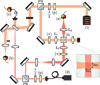 |
Fig. 1 Schematic of the experimental setup. (1) Pump laser (pulsed Nd:YAG). (2) Probe laser (cw frequency tunable diode). (3) Sample (liquid acetone). (a), (b) and (c) Probe, pump and beating signal photodiodes; (p) linear polarizer; (v) vertical polarizer; λ∕2: half-wave plate; PB: Polarizing beamsplitter; L1, L2 and L3 : 50 mm, 50 mm and 75 mm focal length lenses. |
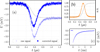 |
Fig. 2 (a) Temporal profile of the raw and the corrected probe signals (points) and fit of the variation of intensity of the raw signal due to thermal lensing (dashed curve). (b) Temporal profile of the pump laser (solid curve) and integration of the temporal profile (dashed curve). (c) Temporal profile of the probe signal on ms timescale. |
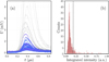 |
Fig. 3 (a) Raw signals detected with photodiode (a) in the absence of probe laser beam due to the scattering of the pump laser, light gray signals correspond to the 15% of highest intensity background signals and are not considered to determine the Brillouin gain signal (see text). (b) Statistics of the intensity of the scattering signal (realized over a set of 500 signals),events to the right of the dotted line correspond to the 15% highest intensity background signals. |
3 Experimental results and discussion
The experimental results showing the measurement of the g(Ω) function of liquid acetone at room temperature in a confined spatio-temporal domain are shown in Figure 4. As expected, the Brillouin gain is negative for Ω < 0 and positive for Ω > 0. Even with important background signals inherent to this confined configuration, the SNR of the Brillouin gain spectrum is satisfying.
We have fitted both the positive and negative frequency region with a Lorentzian function given by:
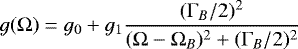 (3)
(3)
with ΩB the central angular frequency, ΓB the full width at half maximum, g1 the line-center gain factor, g0 the additional offset due to background fluctuations discussed in previous section. The values of the fit parameters are given in Table 1.
The values obtained for the central angular frequency ΩB (2.144 GHz and 2.143 GHz) are consistent with the ones measured by Ratanaphruks et al. using a cw SBG spectrometer [23], who found ΩB ∕2π = 5.05 ± 0.01 GHz for a laser excitation of 632.8 nm and a scattering angle of ~178°. More precisely, if using equation (1) one transposes the result of Ratanaphruks et al. to our central laser wavelength (1064 nm) and a scattering angle of 90°, one finds that the corresponding Brillouin frequency is ΩB ∕2π = 2.124 ± 0.004 GHz. Doing so with the results of experiments using either spontaneous Brillouin scattering or SBS in the generator configuration, one finds: 2.12 GHz [4,24], 2.14 GHz [25]. Reference [26] measured the temperature dependence of the Brillouin frequency of liquid acetone. For λ = 1064 nm and θ = 90°, it is−11 MHz/K around 20 °C. All mentioned measurements agree within a 2 °C definition of “room temperature”2. Another source of dispersion of experimental results is the dependence of the Brillouin frequency on the scattering angle (20 MHz/° at 90° and 1064 nm).
Considering now the full width at half maximum in reference [23], Ratanaphruks et al. gives for acetone at room temperature ΓB ∕2π = 260 ± 10 MHz. The Brillouin linewidth is expected to be proportional to the square of the excited phonon wave vector ΓB ∝q2 [2] where the phonon wave vector is given by q = k1 −k2 with k1 and k2 being the pump and probe wave vectors. The transcription of the 260 MHz Brillouin linewidth to our laser wavelength and geometry gives an expected Brillouin linewidth of 47 MHz much smaller than the linewidth we do measure. A possible explanation of this difference is the following. Let us call tp = 2π∕ΓB the phonon lifetime and Λ = vtp the coherence length of the density grating created by the SBS effect, where v is the speedof sound in acetone. In the contra-propagating geometry of reference [23]: Λ ≪ L∕2, where L is the interaction length between the lasers, and L∕2 corresponds to the average distance crossed by the phonons, created everywhere in the interaction zone. Consequently, the linewidth is dictated by v∕Λ. In our case however, if we take ΓB∕2π = 47 MHz, we find Λ ~ 30 μm and hence Λ > L∕2. Then the crossing time of the phonons is shorter than the phonon lifetime, which consequence is to enlarge the measured linewidth. In this relatively simple picture, we must invoke an effective interaction length of about 15 μm to explain our 80 MHz linewidth measurement, which is indeed of the order of L∕2. A more detailed study of this phenomenon could be of interest but is out of the scope of this work.
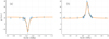 |
Fig. 4 Stimulated Brillouin gain spectrum of liquid acetone at room temperature measured in a confined spatio-temporal domain (30 μm, 170 ns). (a) Ω < 0; (b) Ω > 0. Crosses: experimental data and corresponding error bars; solid curve: fit according to equation (3). Pump and probe lasers central optical wavelength is 1064 nm and their crossing angle is ~ 90°. |


4 Conclusion
We have obtained the Stimulated Brillouin gain spectrum of liquid acetone at room temperature in a narrow spatio-temporal domain (30 μm, 170 ns). This was done using a pulsed SBG spectrometer in a ~ 90° crossing beam geometry. Although there are important sources of background signals inherent to that confined geometry, we were able to accurately measure the Brillouin frequency of the test sample. It agrees well with previous measurements using a cw SBG spectrometer in the contra-propagating geometry or spontaneous Brillouin spectrometers once small variations due to the determination of the scattering angle or of the temperature sample are considered. However these cannot explain the discrepancy between ourmeasurement of the Brillouin linewidth and previous measurements. We believe that the explanation of this difference lies in the occurrence of finite size effects of the acoustic grating produced by SBS in our very confined spatial geometry. We plan to use this SBG spectrometer to investigate the speed of sound in the low density metastable states of liquid 4He [27] produced by a MHz converging acoustic wave [28] where metastable states last for less than 1 μs (acoustic period) and are produced on a spatial scale of less than 100 μm (acoustic focus). In that peculiar situation, the confined spatio-temporal domain SBG spectrometer is very well adapted to assess the acoustic properties of the medium under rapid and local excitation in which thermal phonons are scarce but we are confident that this narrow spatio-temporal SBG spectroscopy can be useful for other situations possibly in the context of applying SBG spectroscopy to biological samples.
Author contribution statement
All the authors have equally participated in building the experimental set up, collecting the data and analyzing the results. All the authors were involved in the preparation of the manuscript and have read and approved the final manuscript.
Acknowledgements
We are grateful to T. El Atmani and L. Perennes for their assistance on the diode laser current supply and temperatureregulation, to A. Leclerc and S. Ismael for their help on mechanics, to A. Gohlke and M. Ta for order management, and to L. Grucker for his advice on the crossing beam set up.
References
- L. Brillouin, Ann. Phys. 9, 88 (1922) [Google Scholar]
- R.W. Boyd, Nonlinear Optics, 3rd edn. (Academic Press, Inc., Orlando, FL, 2008) [Google Scholar]
- R.Y. Chiao, C.H. Townes, B.P. Stoicheff, Phys. Rev. Lett. 12, 592 (1964) [Google Scholar]
- D. Pohl, W. Kaiser, Phys. Rev. B 1, 31 (1970) [Google Scholar]
- S.Y. Tang, C.Y. She, S.A. Lee, Opt. Lett. 12, 870 (1987) [CrossRef] [PubMed] [Google Scholar]
- W.T. Grubbs, R.A. MacPhail, Rev. Sci. Instrum. 65, 34 (1994) [Google Scholar]
- I. Remer, A. Bilenca, Opt. Lett. 41, 926 (2016) [CrossRef] [PubMed] [Google Scholar]
- C.W. Ballmann, J.V. Thompson, A.J. Traverso, Z. Meng, M.O. Scully, V.V. Yakovlev, Sci. Rep. 5, 18139 (2015) [CrossRef] [PubMed] [Google Scholar]
- D. Bedborough, D. Jackson, Polymer 17, 573 (1976) [Google Scholar]
- J.M. Vaughan, J.T. Randall, Nature 284, 489 (1980) [Google Scholar]
- K.J. Koski, J.L. Yarger, Appl. Phys. Lett. 87, 061903 (2005) [Google Scholar]
- G. Scarcelli, S.H. Yun, Nat. Photon. 2, 39 (2008) [CrossRef] [PubMed] [Google Scholar]
- G. Scarcelli, S.H. Yun, Opt. Express 20, 9197 (2012) [CrossRef] [PubMed] [Google Scholar]
- Z. Meng, A.J. Traverso, C.W. Ballmann, M.A. Troyanova-Wood, V.V. Yakovlev, Adv. Opt. Photon. 8, 300 (2016) [CrossRef] [Google Scholar]
- C.W. Ballmann, Z. Meng, V.V. Yakovlev, Biomed. Opt. Express 10, 1750 (2019) [CrossRef] [PubMed] [Google Scholar]
- C.Y. She, G.C. Herring, H. Moosmüller, S.A. Lee, Phys. Rev. Lett. 51, 1648 (1983) [Google Scholar]
- G.W. Faris, L.E. Jusinski, M.J. Dyer, W.K. Bischel, A.P. Hickman, Opt. Lett. 15, 703 (1990) [CrossRef] [PubMed] [Google Scholar]
- G.W. Faris, L.E. Jusinski, A.P. Hickman, J. Opt. Soc. Am. B 10, 587 (1993) [Google Scholar]
- G.W. Faris, M. Gerken, C. Jirauschek, D. Hogan, Y. Chen, Opt. Lett. 26, 1894 (2001) [CrossRef] [PubMed] [Google Scholar]
- W.T. Grubbs, R.A. MacPhail, J. Chem. Phys. 97, 19 (1992) [Google Scholar]
- P.J. Linstrom, W.G. Mallard, J. Chem. Eng. Data 46, 1059 (2001) [Google Scholar]
- D. Beysens, P. Calmettes, J. Chem. Phys. 66, 766 (1977) [Google Scholar]
- K. Ratanaphruks, W.T. Grubbs, R.A. MacPhail, Chem. Phys. Lett. 182, 371 (1991) [Google Scholar]
- M. Denariez, G. Bret, Phys. Rev. 171, 160 (1968) [Google Scholar]
- H.Z. Cummins, R.W. Gammon, J. Chem. Phys. 44, 2785 (1966) [Google Scholar]
- D.P. Eastman, A. Hollinger, J. Kenemuth, D.H. Rank, J. Chem. Phys. 50, 1567 (1969) [Google Scholar]
- J. Grucker, J. Low Temp. Phys. 197, 149 (2019) [Google Scholar]
- A. Qu, A. Trimeche, J. Dupont-Roc, J. Grucker, P. Jacquier, Phys. Rev. B 91, 214115 (2015) [Google Scholar]
Determined from our measurement of the absorption coefficient of liquid acetone at 1064 nm, α ~ 0.5 m−1, and from the density and specific heat of liquid acetone [21].
Note that the local heating of our sample of about tenths of mK changes the Brillouin frequency of only hundreds of kHz.
Cite this article as: Lionel Djadaojee, Albane Douillet, Jules Grucker, Stimulated Brillouin gain spectroscopy in a confined spatio-temporal domain (30 μm, 170 ns), Eur. Phys. J. Appl. Phys. 89, 30701 (2020)
All Tables
All Figures
|
Fig. 1 Schematic of the experimental setup. (1) Pump laser (pulsed Nd:YAG). (2) Probe laser (cw frequency tunable diode). (3) Sample (liquid acetone). (a), (b) and (c) Probe, pump and beating signal photodiodes; (p) linear polarizer; (v) vertical polarizer; λ∕2: half-wave plate; PB: Polarizing beamsplitter; L1, L2 and L3 : 50 mm, 50 mm and 75 mm focal length lenses. |
| In the text | |
|
Fig. 2 (a) Temporal profile of the raw and the corrected probe signals (points) and fit of the variation of intensity of the raw signal due to thermal lensing (dashed curve). (b) Temporal profile of the pump laser (solid curve) and integration of the temporal profile (dashed curve). (c) Temporal profile of the probe signal on ms timescale. |
| In the text | |
|
Fig. 3 (a) Raw signals detected with photodiode (a) in the absence of probe laser beam due to the scattering of the pump laser, light gray signals correspond to the 15% of highest intensity background signals and are not considered to determine the Brillouin gain signal (see text). (b) Statistics of the intensity of the scattering signal (realized over a set of 500 signals),events to the right of the dotted line correspond to the 15% highest intensity background signals. |
| In the text | |
|
Fig. 4 Stimulated Brillouin gain spectrum of liquid acetone at room temperature measured in a confined spatio-temporal domain (30 μm, 170 ns). (a) Ω < 0; (b) Ω > 0. Crosses: experimental data and corresponding error bars; solid curve: fit according to equation (3). Pump and probe lasers central optical wavelength is 1064 nm and their crossing angle is ~ 90°. |
| In the text | |
Current usage metrics show cumulative count of Article Views (full-text article views including HTML views, PDF and ePub downloads, according to the available data) and Abstracts Views on Vision4Press platform.
Data correspond to usage on the plateform after 2015. The current usage metrics is available 48-96 hours after online publication and is updated daily on week days.
Initial download of the metrics may take a while.