| Issue |
Eur. Phys. J. Appl. Phys.
Volume 98, 2023
|
|
|---|---|---|
| Article Number | 65 | |
| Number of page(s) | 16 | |
| Section | Plasma, Discharges and Processes | |
| DOI | https://doi.org/10.1051/epjap/2023230072 | |
| Published online | 20 December 2023 | |
https://doi.org/10.1051/epjap/2023230072
Original Article
Interpretation of temperature measurements by the Boltzmann plot method on spatially integrated plasma oxygen spectral lines
LAPLACE, Université de Toulouse, CNRS, INPT, UPS, Toulouse, France
* e-mail: This email address is being protected from spambots. You need JavaScript enabled to view it.
Received:
31
March
2023
Received in final form:
8
September
2023
Accepted:
20
October
2023
Published online: 20 December 2023
Abstract
In thermal plasma spectroscopy, the Boltzmann plot method is particularly popular for measuring plasma temperature independently of pressure. In order to better understand the results of the Botzmann plot measurements performed with atomic oxygen lines on our thermal plasma, which has a non-negligible thickness, a Python code was developed based on the assumption of local thermodynamic equilibrium (LTE) and the calculated plasma composition and properties. This code allows us to simulate a measurement of the oxygen line intensity resulting from an integration over the plasma thickness in a chosen direction for a given temperature profile. From these a simulated Boltzmann plot gave us a simulated temperature. It resulted that this measurement is governed by the maximum of the temperature profile until the maximum temperature exceeds that of the maximum emissivity of the atomic oxygen lines. Above that temperature a limitation was observed, it is possible to measure higher temperatures but the interpretation of that measurement is difficult. Plasma pressure has a limited effect on this limitation. When no limitation is observed, the temperature measurement from the Boltzmann plot method that we simulated is always at least 90% of the maximum of the temperature profile.
© J. Thouin et al., Published by EDP Sciences, 2023
 This article is distributed under the terms of the Creative Commons Attribution License https://creativecommons.org/licenses/by/4.0 which permits unrestricted use, distribution, and reproduction in any medium, provided the original author(s) and source are credited.
1 Introduction
The Boltzmann plot method is widely used to determine the temperature of plasmas by emission spectroscopy [1–8].
This method is particularly popular because it is not as experimentally demanding as, for example, absolute intensity measurements and allows a temperature to be determined independently of pressure. However, it requires the plasma to be in local thermodynamic equilibrium and is often subject to significant uncertainties.
There are spectroscopic acquisition methods that allow spatial resolution of the measurement. They can be based on an axisymmetry assumption like Abel inversion [4,5] or not, like tomographic reconstruction methods [9]. However, quite often, the measurement carried out is spatially integrated [1,3,6–8], which raises the question of the interpretation of this measurement. When light is collected using a collimation system or directly from an optical fiber, it is integrated over the entire thickness of the plasma which is not homogeneous in temperature. The Boltzmann plot method is then performed on the different spectral lines resulting from that integration.
The presented study was carried out in order to interpret experimental results of Boltzmann plot temperature measurement based on atomic oxygen spectral lines emitted by a water thermal plasma. This plasma, considered at local thermodynamic equilibrium (LTE), is generated by a ten milliseconds electric arc in a water tank that vaporizes the water. Pulsed electro-hydraulic discharges have many applications in metal forming, rock pulverization and water purification [10–12].
The three lines we are using experimentally are presented in Table 1, they have also been used on a similar laser induced plasma by Hannachi et al. [15]. These lines were chosen because they were the only ones observed that allowed temperature measurements using a Boltzmann plot method.
In this study authors have shown that self-absorption of the 777 nm line in particular can be quite important. However, because self-absorption is very specific to the plasma under study, we will not consider self-absorption effects in this article, but recommend that these effects be corrected on the experimental measurements. These corrections can be achieved using escape factors on the intensity measurements, the method is presented in [15].
2 Context
We performed experimental emission spectroscopy measurements on a water plasma. The details of the experimental setup used to generate the arc are presented in Thouin et al. [16]. The electric arc generates a water vapor bubble within the liquid water and light can be collected for slightly less than 10 ms (see Fig. 1). In order to determine a plasma temperature using Boltzmann plot method we had to capture three emission spectral lines of the same element with different upper transition state energies. We decided to use three emission lines of the atomic oxygen that will be presented in Section 3.
To illustrate, Figure 1 shows the observed bubble with the plasma contained in the saturated zone. This image was obtained using a Photron FASTCAM SA5 high-speed camera, the exposure time was 1/25000 s and three neutral density filters were fitted on the lens with an attenuation factor respectively of 64, 32 and 16. The acquisition method is described with more details in [17]. A halogen lamp is used as backlighting. Backlighting is only necessary to improve the observation of the edge of the water vapor bubble. The arc is generated between two tungsten rods of 1.6 mm diameter placed vertically and ignited using a 0.13 mm diameter copper wire acting as a fuse. Pulse duration is about 10 ms for a total energy deposited of a few kJ. On Figure 1 the bubble's radius is at its maximum and is about 2.5 cm and the warm core of the plasma on the right is about 5 mm in diameter.
When considering no self-absorption, the light collected is the sum of all emissions on the line of sight selected by the two pinholes, see Figure 2.
Figure 2 shows the light being collected on the line of sight I(X0). We will consider that the profile of one emission spectral line, at a given wavelength, integrated along the line of sight over the entire plasma thickness is the sum of the local emissions at that same wavelength along the line of sight. These local emission spectral lines can be characterized using the local conditions of emission. We will describe this process in Section 4.1.
A theoretical study of the phenomenon was carried out in our team [18] in order to understand the behavior of the plasma. A water plasma bubble was simulated using the commercial @Fluent software. Plasma properties have been calculated for water, the theory is presented in Harry-Solo et al. [19]. This study gave us a homogenous value for the pressure inside the vapor bubble close to 3 bar at very early times of the expansion (t < 0.5 ms). Therefore, in this article, the plasma will be considered to be pure water and its properties calculated for a pressure of 3 bar.
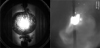 |
Fig. 1 Image of a water vapor bubble (left), the image is saturated in the center by the emission of light from the arc [16]. Close up image of the plasma (right) using a band-pass optical filter centered on the Hα hydrogen spectral line. |
3 Spectral emission line description
The emissivity associated with an electronic transition from an energy level i to an energy level j is expressed as:
 (1)
(1)
with:
J(λ) emissivity profile as a function of the wavelength.
ni population density of the emitting level i.
Aij Einstein coefficient for the electronic transition from level i to j.
P, T pressure and temperature.
h, c Planck's constant and speed of light in vacuum.
If the plasma is assumed to be at local thermodynamic equilibrium (LTE) then the density ni of the level i is given by Boltzmann law:
 (2)
(2)
with:
n(P,T) global species density: n (T, P) = ∑k nk with k being the excitation level.
Z(P,T) partition function for the considered species.
Ei energy for the level i.
gi degeneracy of the level i.
K: Boltzmann constant.
The emissivity can be expressed as:
 (3)
(3)
And λt is the wavelength of the light emitted by the electronic transition considered.
To construct the Boltzmann plot, equation (3) is linearized using the logarithm function. This leads to the following equation:
 (4)
(4)
Jtot(W/m2) is the spectral radiance integrated over the line profile. The logarithm being a transcendental function both sides of equation (3) should be normalized to the unit radiance  can all be taken equal to unity; this does not affect the temperature measurement but it assures that the terms in the logarithms are dimensionless. The temperature measurement comes from the last term of equation (4) which is dimensionless, it is the slope of the plot and is unaffected by the normalization of the emissivity. This is explained in details in Völker et al. [20].
Table 1 shows the characteristics of the three atomic oxygen spectral lines chosen to perform the Boltzmann plot.
The emissivity Jtot depends on the pressure and the temperature. Z(P,T) and n(P,T) have been calculated, using a program developed in the team, for pure water for temperatures ranging from 300 K to 60 000 K at 3, 5 and 10 bar. For a thermal plasma considered to be in LTE, solving the corresponding equations (Saha-Eggert, Guldberg-Waage, electrical neutrality, Dalton law) gives us the evolution of the plasma species densities as a function of pressure and temperature. The method for calculating the properties is presented in Harry-Solo et al. [19].
Figure 3 shows that the 777.3 nm atomic oxygen triplet has the highest emissivity and the 715.7nm has the lowest one. The maximum emissivity is reached around 17 kK for the 777.3 and 844.6 nm spectral lines and 18.5 kK for the 715.7 nm line.
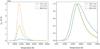 |
Fig. 3 Emissivity Jtot for the three OI spectral lines as a function of temperature for pure water at 3 bar; on the left in arbitrary unit and on the right all three maxima normalized to unity in order to visualize the temperature for each maximum. |
4 Results
4.1 Temperature profiles with different shapes and temperature maxima
We seek to reconstruct, for several temperature profiles, the spectral lines emission in a manner similar to what we observe experimentally. Each of the three OI spectral lines is integrated over the plasma thickness and we have to calculate the emissivity at each point along the path of the integrated light (see Fig. 2). For a given spectral line it is dependent on the local conditions of emission, in that case the temperature and the pressure. We consider a pure water plasma with a constant pressure (3 bar).
To construct the Boltzmann plot method, we only need the resulting spatially integrated emissivity of each line. This means that unlike our previous work on Stark broadening of the Hα spectral line [16] we do not need to reconstruct the line profile.
In this section, we will use the different temperature profiles previously defined in Thouin et al. [16] for a similar study on Stark broadening of the Hα spectral line. These temperature profiles are presented on Figure 4. The temperature profiles were defined with a maximum temperature in the center.
The purpose of using several temperature distribution profiles is to draw general conclusions for this temperature measurement and then interpret measurements made in the absence of information on the temperature distribution.
The reconstruction of the three OI spectral lines emissions as well as the construction of the associated Boltzmann plot and the determination of the temperature was performed numerically using an in-house developed Python program. For each line, the total emissivity used for the plot is a sum over the temperature profile of the local emissivity.
 (5)
(5)
with Jk the simulated integrated emissivity for the spectral line k.
Figure 5 shows that these simulated emissivities are well aligned on the Boltzmann plot and the interpolated fit allows us to determine the slope and therefore the temperature. All temperature profiles were processed using this method and the results are shown in Figures 6 and 7.
We observe on Figure 6 that the temperature resulting from the Boltzmann plot method simulated measurement is close to that of the maximum temperature for all profiles. The lowest measured temperature is 14.2 kK for profile P4, which is not the profile with the lowest average temperature but it is the “pointiest” profile, i.e., the profile where the warm zone in the center is the thinnest and most rapidly decreasing as you move away from the center. On the other hand, it is for profile P3 that the temperature measured is the highest with 15 kK. It is also the profile with the most widespread center warm zone. All this seems to indicate that the temperature resulting from the simulated measurement seems to be driven in greater part by the hottest area (which is the most emissive area) than by the other parts of the profile. This can also be observed when comparing profiles P1 and P2, which are both Gaussian temperature profiles with a similar maximum temperature but different width. Differences are the peripheral regions of the plasma where profile P2 is warmer as it is defined by a wider Gaussian profile, but interestingly there is almost no difference in the simulated temperature measurement.
All profiles but the highly unrealistic fourth profile show a simulated temperature measurement greater than 90% of the maximum temperature of the profile, with the fourth profile just shy of 90%.
In order to extend these results to asymmetric plasmas we used two highly asymmetric temperature profiles and performed the same simulation on them. The results are presented in Figure 7.
Figure 7 shows that the simulated temperature measurement is still over 90% of the profile's maximum for the two asymmetric profiles PA1 and PA2. It is 93% for profile PA2, this is not surprising given that it is a combination of profiles P1 and P2. It is also 93% for profile PA1 which is the combination of profiles P3 and P4, indicating again that the warmest zones of the profile are the most influential on the measurement. Indeed, the measurement for profile PA1 is very close to that of profile P3 which has the largest center warm zone and is almost unaffected by the part of the profile coming from P4 which is the complete opposite.
Temperature profiles 5 to 8 (Fig. 8) are all Gaussian temperature profiles with identical full width at half-maximum and increasing temperature maximum. For profiles P5 and P6 the temperature resulting from the Boltzmann plot method simulated measurement is still over 90% of the maximum profile temperature. However, for profile P7 and even more so for profile P8, although it is still increasing, the temperature of the simulated measurement represents a smaller proportion of the maximum temperature of the profile.
Given that these temperature profiles come from a similar study for Stark broadening of the Hα spectral line [16] it is interesting to compare the results of the different simulated measurements. In Thouin and al. [16] Stark broadening simulated measurements give the electronic density. However, the plasma was considered with a homogenous pressure of 3 bar and we can therefore give a corresponding temperature to the electronic density measurement using plasma composition. Results for the ten profiles are given in Table 2.
These results suggest that for this Gaussian profile shape, there is a limit to the temperature measurement. In order to verify this, we will study Gaussian profiles with higher maximum temperature in the following section.
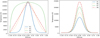 |
Fig. 4 (Left) the first four profiles have different shape and a similar temperature maximum (≈16 kK); (Right) the last four profiles are Gaussian temperature profiles presenting identical width at half height but different maxima. [16]. |
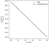 |
Fig. 5 Boltzmann plot with the simulated integrated emissivity of the three OI spectral lines for the temperature profile P1 (see Fig. 4). |
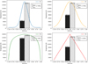 |
Fig. 6 Temperature profiles P1-4 (hatched in black is the mean temperature over the profile and hatched in white is the temperature resulting from the Boltzmann plot method simulated measurement). |
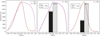 |
Fig. 7 Temperature profiles PA1 and PA2 [16]. Results: hatched in black is the mean temperature over the profile and hatched in white is the temperature resulting from the Boltzmann plot method simulated measurement. |
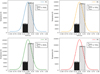 |
Fig. 8 Temperature profiles P5-8 (hatched in black is the mean temperature over the profile and hatched in white is the temperature resulting from the Boltzmann plot method simulated measurement). |
4.2 Different values of the temperature maximum
We have defined four Gaussian temperature profiles with full width at half-maximum identical to that of profiles P4-8 of Section 4.1 but with considerably larger temperature maxima. These profiles are presented in Figure 9.
Figure 10 shows the results of the simulated measurements.
Simulated Boltzmann temperature measurements made on profiles P1-4 (Fig. 10) show not only that there is a limit to the temperature that can be measured with this shape of temperature profile, but also that the maximum temperature measured is not for the hottest profile. The highest temperature measured is the one carried out on profile P2 and it decreases on profiles P3 and P4. Of course, the temperatures, especially for the P3 and P4 profiles, greatly exceed the temperatures of the emissivity maximum for the atomic oxygen lines. In this section it allows us to visualize a limitation of the measurement and in Section 4.5 we will discuss the spectral lines expected at these temperatures.
In order to get a more accurate picture of this limit for the simulated temperature measurement, we ran the simulation on a larger number of Gaussian profiles, keeping the same FWHM and varying the maximum temperature. Results are presented on Figure 11, showing the simulated measurement relative to the maximum of the temperature profile.
The simulated temperature measurements presented in Figure 11 clearly show a limitation, the maximum measured temperature is 19.1 kK for a profile's maximum of 30.8 kK. The simulated measurement behaves differently depending on whether it is below or above the temperature limit. For relatively low profile's maximum temperature the simulated measurement is pretty close to that maximum (above 95%) and then around a profile's maximum temperature of 18 kK, where the simulated Boltzmann temperature measurement is still around 95% of that maximum, that percentage starts to decrease more rapidly. In the following section, we will question whether this limitation is dependent on plasma pressure.
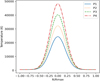 |
Fig. 9 Gaussian temperature profiles presenting identical widths at half height but different maxima. |
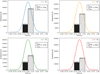 |
Fig. 10 Temperature profiles P1-4 (hatched in black is the mean temperature over the profile and hatched in white is the temperature resulting from the Boltzmann plot method simulated measurement). |
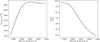 |
Fig. 11 (Left): Temperature resulting from the Boltzmann plot method simulated measurement as a function of the maximum temperature of the corresponding Gaussian profile. (Right): Percentage of the profile's maximum that the simulated temperature measurement represents as a function of the profile's maximum temperature. |
4.3 Different values of plasma pressure
It is important to note that the Boltzmann plot method provides a temperature measurement independent of the pressure of the plasma under LTE assumption. We are not seeking to determine whether the plasma pressure affects the simulated measurement but rather to establish whether the pressure affects the limitation we observe on that measurement. Although the results are not shown here, all profiles that have been tested for a plasma at 3 bar (including those from the following section) have also been tested at 5 and 10 bar and, when no limitation is observed, there is little to no difference in the simulated Boltzmann temperature measurement.
The temperature limit is close to that of the maximum emissivity for the three OI spectral lines we are using to build the Boltzmann plot. If this limitation is due to the maximum emissivity temperature, then it should be affected by a change in plasma pressure.
At 5 bar, the maximum emissivity is reached around 17.5 kK for the 777.3 and 844.6 nm spectral lines and 19 kK for the 715.7 nm line. At 10 bar it is around 18.5 kK for the spectral lines at 777.3 and 844.6 nm and 20 kK for the 715.7 nm line (see Fig. 12). According to these results, if the limitation of the temperature measurement is related to the maximum emissivity temperature of the spectral lines, a pure water plasma at a higher pressure would only allow slightly higher temperatures to be measured. Similarly, to the previous section, we ran the simulation on a larger number of Gaussian profiles, keeping the same FWHM and varying the maximum temperature. Results are presented on Figure 13.
The limitation we observed on Figure 11 for a plasma at 3 bar is still present at 5 and 10 bar (see Fig. 13). Overall, the behavior of the Boltzmann simulated measurement is very similar for 3, 5 and 10 bar water plasmas. As expected, as the pressure increases, the maximum measured temperature increases slightly. The maximum temperature measured is approximately 19.9 kK at 5 bar and 20.9 kK at 10 bar. These results show that there is a connection between the maximum emissivity of the spectral lines and the measurement limitation. The limit of the temperature measurement, both at 5 and 10 bar, is slightly above that of the maximum emissivity of the 715.7 nm spectral line. This was also true at 3 bar (see Figs. 3 and 11).
Unfortunately, these results do not explain how it is possible to achieve temperature measurements above 20 kK, temperatures that we believe can be measured with these atomic oxygen lines based on experimental results. In the next section, we will use temperature profiles where the central warm zone is wider than any of the previous profiles, in order to see if it is possible to measure temperatures considerably higher than the temperature limit we have met until then.
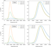 |
Fig. 12 Emissivity Jtot for the three OI spectral lines as a function of temperature for pure water (top) at 5 bar, (bottom) at 10 bar. |
 |
Fig. 13 Results for pure water plasma (top) at 5 bar, (bottom) at 10 bar. (Left) temperature resulting from the Boltzmann plot method simulated measurement as a function of the maximum temperature of the corresponding Gaussian profile. (Right) Percentage of the profile's maximum that the simulated temperature measurement represents as a function of the profile's maximum temperature. |
4.4 Wider Gaussian temperature profiles
As the effect of pressure on the Boltzmann temperature measurement was discussed in the previous section, the following results will only be presented for a 3 bar plasma.
The temperature profiles presented on Figure 14 were all chosen with a maximum of approximately 32 kK. P1 and P2 are Gaussian with a width at half maximum larger than any previous profile. P3 and P4 are designed to maximize the warm centre part of the profile and were inspired by profile P3 from Section 4.1 since this was the profile with the highest temperature measured for a given maximum. Results of the simulated measurements are presented on Figure 15.
The simulated Boltzmann temperature measurements for the first two profiles P1 and P2 are still affected by the limitation, despite the significant increase in width at half height. Profile P3 and profile P4 even further enabled a simulated measurement that exceeded the limit value we observed until then for Gaussian profiles. These last two profiles showed that it was possible for some profiles to exceed the temperature limit that we had previously observed on the simulated measurement and, in doing so, it also showed that it was possible to measure temperatures exceeding that of the maximum emissivity of the spectral lines used for the Boltzmann plot. The simulated temperature measurement is 71 % of the maximum temperature of the profile for profile P3 and 77% for profile P4. Unfortunately, once the temperature limit is exceeded (simulated measurement over 20 kK) it is very difficult to get an idea of the profile's maximum temperature without knowing the profile's shape. To better illustrate this, we studied two additional profiles and the results are presented on Figure 16.
Perhaps surprisingly, Figure 16 shows that the simulated temperature measurement is lower for profile P6 even though it is warmer than profile P5 and they have the same shape. With profile P6, the warm central part of the profile with a temperature of approximately 40 kK, is less emissive for the three oxygen spectral lines than the same part for profile 5 with approximately 32 kK. Therefore, the measurement is “pulled” by the area of maximum temperatures to a larger extent for profile 5 than for profile 6.
These results show that if a temperature measurement is made near 24 kK as is the case for profile P6 and without information on the shape of the profile, we are unable to determine maximum temperature of the profile. It is not possible to know whether it is a profile with a maximum temperature much warmer than the measurement and a very quick temperature drop in the peripheral parts of the profile or a profile closer to profile P4 with a maximum only slightly warmer than 24 kK.
The atomic oxygen lines used for the Boltzmann plot show a significant decrease in emissivity at high temperatures (well above 30 kK). For these temperatures, other spectral lines will be observed, notably OII lines which progressively replaces atomic oxygen in the plasma as the temperature increases. This will be discussed in detail in the next section.
 |
Fig. 14 The first two profiles are Gaussian temperature profiles with increasing width at half height, profile number three and four are inspired of profile P3 from Section 4.1. |
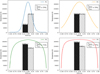 |
Fig. 15 Temperature profiles P1-4 (hatched in black is the mean temperature over the profile and hatched in white is the temperature resulting from the Boltzmann plot method simulated measurement). |
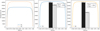 |
Fig. 16 Temperature profiles P5 and P6. Results: hatched in black is the mean temperature over the profile and hatched in white is the temperature resulting from the Boltzmann plot method simulated measurement. |
4.5 Temperature indication given by other spectral lines
One possibility to get an indication of the temperature range is to observe other spectral lines emitted by the plasma. The lines that will be of interest are lines whose transition's upper energy level is higher than that of the lines used for the Boltzmann plot. In this case, the emissivity of the observed lines must be calculated as a function of temperature and pressure. When no such lines are observed, it is then necessary to identify lines that might be observed if the conditions allowed it. In our case, the presence or absence of certain OII emission lines can give us an indication of the plasma temperature. We decided to study the emissivity of an OII spectral line that is a strong line of oxygen. This line at 464.18 nm was observed by Sember et al. [21] in a steam torch plasma. It is a line that could be observed if the atomic oxygen lines considered in this article are present.
Figure 17 shows that the maximum emissivity for that line is around 34 kK at 3 bar and 37 kK at 10 bar. It is considerably more than for the atomic oxygen lines used for the Boltzmann plot. If this OII spectral line is observed then it is very likely that the plasma reaches temperatures above 25 kK. Of course, the absence of a line alone does not show that the plasma temperature is lower. However, if when observing the whole emission spectrum, no lines of higher emitting energy level are observed, this is an indication that the plasma likely does not reach the temperatures required for the emission of these lines.
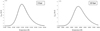 |
Fig. 17 Emissivity Jtot for the 464.18 nm OII spectral line as a function of temperature for pure water (left) at 3 bar, (right) at 10 bar. |
5 Conclusion
In this study we have set out to interpret spectroscopic temperature measurements using the Boltzmann plot method. This method allows a pressure-independent measurement of the temperature of plasmas at local thermodynamic equilibrium. However, when this measurement results from a spatial integration, questions arise about the meaning of this measurement. We set up different temperature profiles of a hypothetical water plasma and for these different profiles we studied the temperatures corresponding to a numerically simulated Boltzmann diagram measurement.
The results of the first profiles (Sect. 4.1) seemed to indicate that the temperature measured by the Boltzmann plot method was dominated by the warm central part of the profile. In fact, this remains true until the maximum temperature of the profile reaches the maximum emissivity temperature of the spectral lines used for the Boltzmann plot. But beyond this limit the temperature measured could hardly increase for the conventional profiles we had defined. We had to define profiles where the warm central part strongly prevails in the profile and where the parts whose temperatures are close to those of the maximum emissivity of the spectral lines, are of very little importance. These results showed that, when the maximum temperature of the profile exceeds the maximum emissivity temperature, the simulated measurement is dominated by the parts of the profile close to this maximum emissivity temperature.
The influence of the plasma pressure is quite small, other than when a limitation of the measurement occurs, the Boltzmann plot method allows a temperature measurement independent of the pressure. When a measurement limitation is observed, the difference between the maximum temperature measured at 3 bar and at 10 bar on Gaussian profiles is only 2 kK. This is fairly small considering that the experimental Boltzmann diagram method is often subject to significant uncertainties.
We have shown that it is however possible to measure temperatures above the maximum emissivity temperature of the spectral lines used to construct the Boltzmann plot for temperature profiles where the warm region (above 20 kK) largely dominates the profile. However, for the profiles we studied (P1-6 Sect. 4.4), the measured temperature does not represent as large a percentage of the profile maximum as it does for colder profiles unaffected by the limitation on the measurement. For these profiles, the measured temperature depends to a larger extent on the temperature distribution in the profile and is therefore more difficult to interpret. The purpose of this study is to give elements of interpretation for spatially integrated temperature measurements based on the Boltzmann plot method when it is impossible to determine the temperature distribution within the plasma.
The results of the simulated measurement on the different profiles where we did not see a temperature limitation allow us to draw a conclusion on the meaning to be given to the Boltzmann spatially integrated temperature measurement. When the temperature measurement from the Boltzmann plot method is made using the oxygen spectral lines we have chosen (see Tab. 1) and is less than 20 kK, no matter what the temperature distribution within the plasma, this measurement corresponds to at least 90% of the maximum temperature of the integrated plasma profile for all tested pressure values.
Conflict of interests
The authors have nothing to disclose.
Funding
This research received no external funding.
Data availability statement
This article has not associated data which could be deposited.
Author contribution statement
JT developed the computer code, carried out the analysis of the results and wrote the manuscript. MB, PF and JJG reviewed the manuscript. PF and JJG provided data for the analysis. JT and PF had the initial idea.
Appendix A
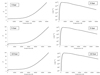 |
Fig. A1 Partition function (left) and density (right) of atomic oxygen OI for pure water at 3, 5 and 10 bar. |
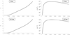 |
Fig. A2 Partition function (left) and density (right) of singly ionized oxygen OII for pure water at 3 and 10 bar. |
References
- V.S. Burakov, E.A. Nevar, M.I. Nedel'ko et al., Spectroscopic diagnostics for an electrical discharge plasma in a liquid, J. Appl. Spectrosc. 76, 856 (2009) [CrossRef] [Google Scholar]
- F. Wang, Y. Cressault, P. Teulet et al., Spectroscopic investigation of partial LTE assumption and plasma temperature field in pulsed MAG arcs, J. Phys. Appl. Phys. 51, 255203 (2018) [CrossRef] [Google Scholar]
- T. Namihira, S. Sakai, T. Yamaguchi et al., Electron Temperature and Electron Density of Underwater Pulsed Discharge Plasma Produced by Solid-State Pulsed-Power Generator, IEEE Trans. Plasma Sci. 35, 614 (2007) [CrossRef] [Google Scholar]
- G. Ni, P. Zhao, C. Cheng et al., Characterization of a steam plasma jet at atmospheric pressure, Plasma Sources Sci. Technol. 21, 015009 (2012) [CrossRef] [Google Scholar]
- A. Mašláni, V. Sember, M. Hrabovský, Spectroscopic determination of temperatures in plasmas generated by arc torches, Spectrochim. Acta. Part B At. Spectrosc. 133, 14 (2017) [CrossRef] [Google Scholar]
- H. Pauna, M. Aula, J. Seehausen et al., Optical Emission Spectroscopy as an Online Analysis Method in Industrial Electric Arc Furnaces, Steel Res. Int. 91, 2000051 (2020) [CrossRef] [Google Scholar]
- T. Namihira, T. Yamaguchi, K. Yamamoto et al., Characteristics of pulsed discharge plasma in water, in 2005 IEEE Pulsed Power Conference, 2005, pp. 1013–1016 [Google Scholar]
- J. Ben Ahmed, N. Terzi, Z. Ben Lakhdar, G. Taieb, Temporal Characterization of a Plasma Produced by Interaction of Laser Pulses with Water Solutions, Laser. Chem. 20, 111 (2002) [CrossRef] [Google Scholar]
- J. Benech, Spécificité de la mise en œuvre de la tomographie dans le domaine de l'arc électrique: validité en imagerie médicale, These de doctorat, Toulouse 3, 2008 [Google Scholar]
- V.S. Balanethiram, G.S. Daehn, Hyperplasticity: Increased forming limits at high workpiece velocity, Scr. Metall. Mater. 30, 515 (1994) [CrossRef] [Google Scholar]
- S. Boev, V. Vajov, B. Levchenko et al., Electropulse technology of material destruction and boring, in Digest of Technical Papers. 11th IEEE International Pulsed Power Conference (Cat. No.97CH36127) (1997), Vol. 1, pp. 220–225 [Google Scholar]
- L. Edebo, I. Selin, The Effect of the Pressure Shock Wave and Some Electrical Quantities in the Microbicidal Effect of Transient Electric Arcs in Aqueous Systems, Microbiology 50, 253 (1968) [Google Scholar]
- A. Hibbert, E. Biemont, M. Godefroid, N. Vaeck, E1 transitions of astrophysical interest in neutral oxygen, J. Phys. B At. Mol. Opt. Phys. 24, 3943 (1991) [CrossRef] [Google Scholar]
- K. Butler, C.J. Zeippen, OSCILLATOR STRENGTHS FOR ALLOWED TRANSITIONS IN NEUTRAL OXYGEN : AN ASSESSMENT OF THE OPACITY PROJECT DATA ACCURACY, J. Phys. IV 01, C1 (1991) [Google Scholar]
- R. Hannachi, P. Teulet, G. Taieb et al., Influence of the self-absorption of atomic lines on the determination of temperature and electron number density in the case of a laser induced cacl2 water plasma, High Temp. Mater. Process. Int. Q High-Technol. Plasma Process. 13, 45 (2009) [Google Scholar]
- J. Thouin, M. Benmouffok, P. Freton, J.-J. Gonzalez, Interpretation of Stark broadening measurements on a spatially integrated plasma spectral line, Eur. Phys. J. Appl. Phys. 97, 87 (2022) [CrossRef] [EDP Sciences] [Google Scholar]
- Z. Laforest, J.J. Gonzalez, P. Freton, EXPERIMENTAL STUDY OF A PLASMA BUBBLE CREATED BY A WIRE EXPLOSION IN WATER, IJRRAS 34, 93 (2018) [Google Scholar]
- Z. Laforest, Etude expérimentale et numérique d'un arc électrique dans un liquide. These de doctorat, Toulouse 3, 2017 [Google Scholar]
- A. Harry Solo, M. Benmouffok, P. Freton, J.-J. Gonzalez, Stochiometry Air – CH4 Mixture: Composition, Thermodynamic Propertiess and Transport Coefficients, PLASMA Phys. Technol. 7, 21 (2020) [CrossRef] [Google Scholar]
- T. Völker, I.B. Gornushkin, Importance of physical units in the Boltzmann plot method, J. Anal. At. Spectrom. 37, 1972 (2022) [CrossRef] [Google Scholar]
- V. Sember, A. Mašláni, P. Křenek et al., Spectroscopic Characterization of a Steam Arc Cutting Torch, Plasma. Chem. Plasma. Process. 31, 755 (2011) [CrossRef] [Google Scholar]
Cite this article as: Julien Thouin, Malyk Benmouffok, Pierre Freton, Jean-Jacques Gonzalez, Interpretation of temperature measurements by the Boltzmann plot method on spatially integrated plasma oxygen spectral lines, Eur. Phys. J. Appl. Phys. 98, 65 (2023)
All Tables
All Figures
|
Fig. 1 Image of a water vapor bubble (left), the image is saturated in the center by the emission of light from the arc [16]. Close up image of the plasma (right) using a band-pass optical filter centered on the Hα hydrogen spectral line. |
| In the text | |
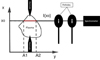 |
Fig. 2 Plasma light selection and acquisition [16]. |
| In the text | |
|
Fig. 3 Emissivity Jtot for the three OI spectral lines as a function of temperature for pure water at 3 bar; on the left in arbitrary unit and on the right all three maxima normalized to unity in order to visualize the temperature for each maximum. |
| In the text | |
|
Fig. 4 (Left) the first four profiles have different shape and a similar temperature maximum (≈16 kK); (Right) the last four profiles are Gaussian temperature profiles presenting identical width at half height but different maxima. [16]. |
| In the text | |
|
Fig. 5 Boltzmann plot with the simulated integrated emissivity of the three OI spectral lines for the temperature profile P1 (see Fig. 4). |
| In the text | |
|
Fig. 6 Temperature profiles P1-4 (hatched in black is the mean temperature over the profile and hatched in white is the temperature resulting from the Boltzmann plot method simulated measurement). |
| In the text | |
|
Fig. 7 Temperature profiles PA1 and PA2 [16]. Results: hatched in black is the mean temperature over the profile and hatched in white is the temperature resulting from the Boltzmann plot method simulated measurement. |
| In the text | |
|
Fig. 8 Temperature profiles P5-8 (hatched in black is the mean temperature over the profile and hatched in white is the temperature resulting from the Boltzmann plot method simulated measurement). |
| In the text | |
|
Fig. 9 Gaussian temperature profiles presenting identical widths at half height but different maxima. |
| In the text | |
|
Fig. 10 Temperature profiles P1-4 (hatched in black is the mean temperature over the profile and hatched in white is the temperature resulting from the Boltzmann plot method simulated measurement). |
| In the text | |
|
Fig. 11 (Left): Temperature resulting from the Boltzmann plot method simulated measurement as a function of the maximum temperature of the corresponding Gaussian profile. (Right): Percentage of the profile's maximum that the simulated temperature measurement represents as a function of the profile's maximum temperature. |
| In the text | |
|
Fig. 12 Emissivity Jtot for the three OI spectral lines as a function of temperature for pure water (top) at 5 bar, (bottom) at 10 bar. |
| In the text | |
|
Fig. 13 Results for pure water plasma (top) at 5 bar, (bottom) at 10 bar. (Left) temperature resulting from the Boltzmann plot method simulated measurement as a function of the maximum temperature of the corresponding Gaussian profile. (Right) Percentage of the profile's maximum that the simulated temperature measurement represents as a function of the profile's maximum temperature. |
| In the text | |
|
Fig. 14 The first two profiles are Gaussian temperature profiles with increasing width at half height, profile number three and four are inspired of profile P3 from Section 4.1. |
| In the text | |
|
Fig. 15 Temperature profiles P1-4 (hatched in black is the mean temperature over the profile and hatched in white is the temperature resulting from the Boltzmann plot method simulated measurement). |
| In the text | |
|
Fig. 16 Temperature profiles P5 and P6. Results: hatched in black is the mean temperature over the profile and hatched in white is the temperature resulting from the Boltzmann plot method simulated measurement. |
| In the text | |
|
Fig. 17 Emissivity Jtot for the 464.18 nm OII spectral line as a function of temperature for pure water (left) at 3 bar, (right) at 10 bar. |
| In the text | |
|
Fig. A1 Partition function (left) and density (right) of atomic oxygen OI for pure water at 3, 5 and 10 bar. |
| In the text | |
|
Fig. A2 Partition function (left) and density (right) of singly ionized oxygen OII for pure water at 3 and 10 bar. |
| In the text | |
Current usage metrics show cumulative count of Article Views (full-text article views including HTML views, PDF and ePub downloads, according to the available data) and Abstracts Views on Vision4Press platform.
Data correspond to usage on the plateform after 2015. The current usage metrics is available 48-96 hours after online publication and is updated daily on week days.
Initial download of the metrics may take a while.