


| Issue |
Eur. Phys. J. Appl. Phys.
Volume 101, 2026
|
|
|---|---|---|
| Article Number | 12 | |
| Number of page(s) | 14 | |
| DOI | https://doi.org/10.1051/epjap/2026008 | |
| Published online | 14 July 2026 | |
https://doi.org/10.1051/epjap/2026008
Original Article
Analytical thermal model for cylindrical DBD reactors: how to obtain a reliable gas temperature distribution, and why is it so important
LAPLACE Laboratory, Université de Toulouse, Toulouse INP, CNRS, 2 rue Charles Camichel, F-31071 Toulouse, France
* e-mail: This email address is being protected from spambots. You need JavaScript enabled to view it.
Received:
19
December
2025
Accepted:
9
June
2026
Published online: 14 July 2026
Abstract
We present a compact analytical thermal model for coaxial dielectric barrier discharge reactors, providing reliable gas-temperature estimates for system-level analysis and design of non-thermal plasma processes; NOₓ abatement is the target of the presented experimental validations. Gas temperature has a major impact on most chemical treatments and is a critical parameter for plasma kinetic solvers (ZdPlaskin in our case for NOₓ abatement efficiency evaluation). Our model couples a volumetric heat source (plasma power deposition) to heat transfer by conduction, convection, and radiation. We validate it experimentally by comparisons across a wide range of power and flow between predicted gas temperatures and measured rotational temperatures obtained from optical emission spectroscopy and between calculated surface temperatures and measured ones obtained by infrared thermography. The model captures very well the main trends and provides temperature estimates with good agreement to the experimental measures. We discuss how the model parameters and outputs can be exported for integration into global chemical kinetics simulations and system-level studies of NOₓ abatement, or any other gas treatment.
Key words: Non-thermal plasma / atmospheric pressure / dielectric barrier discharge / DBD / NOx abatement / thermal modeling / system-level modeling / analytical model / kinetics mechanism / residence time
These authors contributed equally to this work.
© N. Bente et al., Published by EDP Sciences, 2026
 This is an Open Access article distributed under the terms of the Creative Commons Attribution License https://creativecommons.org/licenses/by/4.0 which permits unrestricted use, distribution, and reproduction in any medium, provided the original work is properly cited.
1 Introduction
Nitrogen oxides (NOx) are major atmospheric pollutants, contributing to smog formation, acid rain, and adverse health effects [1–4]. Reducing NOx emissions is therefore a critical environmental and societal challenge, motivating the development of advanced mitigation technologies [5–6]. Among these, non-thermal plasma (NTP) systems—particularly dielectric barrier discharge (DBD) reactors—have shown high NOx removal efficiency [7–12].
As with most chemical processes, the efficiency of plasma-assisted NOx reduction is strongly influenced by temperature. Increasing temperature at constant pressure affects two key aspects of the process: the reduced electric field E/N, via the decrease in gas density N [13,14], and the reaction kinetics, typically governed by Arrhenius-type dependencies [14,15]. These operating conditions also impact residence time: higher temperature reduces gas density, increasing gas velocity for a given mass flow rate. While previous studies [16–18] have examined the influence of reactor geometry or flow conditions, the effect of gas temperature on both kinetics and residence time remains, to our knowledge, largely unexplored for DBD reactors.
Despite its recognized importance, no comprehensive thermal model exists for open-flow, atmospheric-pressure DBD reactors used for NOx reduction. Prior modeling efforts have focused on closed cylindrical DBD configurations [19,20] or plasma actuators for flow control [21] and cannot be directly applied to the reactor topology studied here. This lack of thermal studies likely stems from the experimental difficulty of measuring gas temperature in cold plasmas; validating such models requires advanced diagnostics. In this work, optical emission spectroscopy and infrared (IR) thermography are used to provide the necessary temperature data for model validation.
The main objective of this paper is to present and validate an analytical thermal model of an open-flow, atmospheric-pressure cylindrical DBD reactor for NOx reduction, capable of capturing the influence of gas temperature on both plasma parameters and reactor-scale processes. The paper is organized as follows: Section 2 describes the experimental test bench. Section 3 presents the thermal model, including its assumptions and building of its governing equations. Section 4 details temperature measurement techniques. Section 5 compares model predictions with experimental data from spectroscopy and IR measurements. Section 6 discusses the results and their implications for optimizing non-thermal plasma-assisted processes, i.e., NOx reduction in our case.
2 Experimental setup
The “deNOx” test bench, shown in the schematic diagram of Figure 1, has been developed at LAPLACE laboratory [8,22] to support our experimental investigations. The system consists of a DBD reactor, a gas blending system, a power supply, diagnostics instruments (detailed Sect. 4), and a control interface.
The test bench incorporates three independent DBD reactors mounted along the same cylindrical coaxial quartz structure, with three different lengths of electrodes (metallic meshes with L1 = 6 cm, L2 = 7.7 cm, and L3 = 12.5 cm, used to vary the residence time and power density through changes in reactor geometry) disposed around the outer quartz tube. A single inner electrode, made of 1 mm-thick stainless-steel foil, is inserted inside the inner coaxial quartz tube; its elasticity ensures continuous contact with the tube wall. This design provides optical access for visual observation and spectroscopic diagnostics while maintaining discharge confinement. Detailed dimensions are reported in Figure 1.
The gas blending system consists of three mass flow controllers (MFCs; Bronkhorst EL-Flow Prestige series) regulating the mass flow rates of NO, N2, and O2 injected between the two quartz tubes. Gas cylinders (Air Liquide) with purities above 99.9% for NO and 99.995% for N₂ are used. Upstream MFC pressures are maintained at 4 bar, with atmospheric pressure in the downstream MFC. The gas analyzer (Testo 350) checks the input gas concentration (before the plasma ignition) and evaluates the treatment efficiency (after plasma ignition).
The reactor arrangement has been specifically designed to obtain a laminar flow inside the treatment zone:
Long upstream and downstream distances (gas inlet to treatment zone and treatment to gas outlet: 30 cm) compared with the estimated hydrodynamic and thermal entrance lengths (∼1 cm, according to [23]), so that inlet and outlet disturbances are expected to have relaxed before reaching the treatment zone.
The reactor geometry (1.6 mm gas gap) combined with the gas flow rate provides a Reynolds number (Re ≈ 175 at 10 L/min) well below the turbulent transition limit (Re ≈ 2300).
The flow is, therefore, considered fully laminar in the treatment zone; moreover, the axisymmetric assumption has been set (confirmed by visual observation and thermal camera acquisitions).
The plasma reactor is powered by a custom-built pulsed generator delivering rectangular current pulses to the DBD [8,24,25]. Three independent parameters define the electrical operating conditions: pulse amplitude J, pulse duration Δtp, and switching frequency Fsw. The generator comprises three subsystems: (i) a DC current source controlling J, (ii) a current inverter defining Δtp and Fsw, and (iii) a step-up transformer (turn ratio 1:11) providing the plasma ignition voltage (up to 11 kV). The generator can also operate in “burst mode”, where trains of Non pulses are separated by pauses of Noff inhibited periods, with fully controlled durations. The DBD voltage is measured with a 200 MHz oscilloscope (LeCroy HDO4024) using a 1000:1 probe (Testec TT-SI 9010), while the current is measured with a current probe (Pearson 410).
The test bench is controlled and monitored through a LabVIEW-based supervisor, which controls the operating conditions of each test and guarantees the repeatability of the experiments. The supervisor:
Defines the configuration and set points of controlled Devices (MFCs and power supply);
Sets up and monitors batch experiments (gas mixtures and power supply control);
Handles data acquisition and storage;
Prepares measurements for post-processing and analysis.
The typical operating ranges are summarized in Figure 1. These fully controlled conditions allow parametric studies of the influence of reactor geometry, gas flow rate, and injected electrical power on the reactor temperatures (Sect. 5) and NOx abatement efficiency.
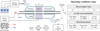 |
Fig. 1 Overview of the “deNOx” test bench. |
3 Temperature’s measurements
3.1 Gas temperature with spectroscopy
Gas temperature inside the treatment zone of the reactor is measured using optical emission spectroscopy. Spectra are recorded with a Princeton Instruments Acton 2500i spectrometer using an 1800 g/mm grating. Light is collected via an optical fiber and a collimator, focused on the external surface of the reactor and aligned along the radial direction (Fig. 2), defining a localized observation region with a diameter of approximately 3 mm. Measurements are performed at five discrete positions along the x-axis (Tab. 1) in order to characterize the axial gradient of the gas temperature. No radial temperature mapping is possible with this experimental setup. All the measurements are performed when thermal steady state is reached (∼10 min). The exposure time is 40 s.
The gas temperature is determined (Eq. 1) from the intensity ratio of two emission lines of the first positive system of  (Fig. 3), according to the method proposed by [26]. The relative uncertainty of the temperature measurement using this method is 10%.
 (1)
(1)
Position of the collimator along the x-axis.
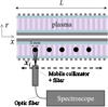 |
Fig. 2 Gas temperature measurement setup. |
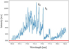 |
Fig. 3 Typical measured spectrum around 774 nm. |
3.2 Surface temperature with IR camera
The surface temperature of the reactor is measured using a FLIR E75 infrared camera (Figs. 4 and 5). Prior to the experiments, the camera is calibrated on a replica of the reactor equipped with thermocouples. An emissivity value of ε = 0.75 is selected to minimize differences between IR readings and thermocouple measurements, resulting in a maximum deviation of 13%. For each experiment, the camera is positioned 40 cm from the reactor, and thermograms are acquired once thermal steady state is reached (approximately 10 min).
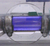 |
Fig. 4 Transversal view of the reactor, taken by the FLIR E75 thermal camera. |
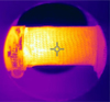 |
Fig. 5 Corresponding thermogram of the reactorsurface recorded at thermal steady state. |
4 Analytical thermal model of the reactor
The current section introduces the modeling hypotheses and details the building of the self-contained model of the cylindrical reactor presented above. It is aimed at reflecting the operating conditions (gas flow and power injection) and providing a prediction of the temperature distribution into the reactor’s volume. All the parameters are introduced in a literal form, allowing this model to be used for parametric investigations.
4.1 Modelling assumptions
The gas mixture flows through the reactor, between the two coaxial quartz tubes, forming a cylindrical annular duct (Fig. 6). The channel is divided into three domains Ω1:
Upstream Ω1 : The gas enters at ambient temperature T0, without plasma interaction.
Reactor Ω2 : The gas temperature increases along the flow direction due to plasma heating.
Downstream Ω3 : The outlet gas cools as it exchanges heat with the surroundings, with its temperature gradually relaxing toward T0.
The model is applicable to the entire duct, but the description below focuses on the reactor region Ω2, where plasma–gas interactions occur. The upstream and downstream regions can be treated analogously, the only distinction being the absence of plasma heating. To enable a tractable analytical formulation, the following assumptions are adopted:
Axisymmetric: All temperatures are invariant with respect to rotation around the reactor axis
 .
.Radial uniformity: Within each material layer (gas, inner wall, and outer wall), the temperature is assumed uniform across the radial direction
 . Hence, the temperatures depend only on the axial coordinate x and time t.
Complete power dissipation: The injected electrical power is assumed to be fully converted into heat. This simplification can be justified through the estimation of the energetic cost of NO removal (6.5 eV per NO molecule dissociated [27]). According to our NO flow rate (max: 10 L/min at atmospheric pressure and ambient temperature), NO removal cost is below 1.7 W. The value is much lower than the electrically injected power: 20–45 W. The remaining power is assumed to be dissipated as heat through collisional relaxation. Our approximation may lead to a slight overestimation because radiative and species transport losses are not considered.
Along the flow direction  , the reactor is discretized into elementary slices of thickness dx (Fig. 7). Each slice is sufficiently thin for the temperature within each material layer to be considered uniform. Three distinct temperatures, shown on Figure 7, are defined for each slice:
 (2)
(2)
Text (x,t) and Tint (x,t): outer and inner quartz walls temperatures; Tg (x,t): gas temperature.
The vector field T(x,t), which gathers these three temperatures, is the output of the thermal model. The following sections describe the equations which are governing the variations of T(x,t) as a function of key operating parameters: gas flow rate, injected electrical power, and reactor geometry.
 |
Fig. 6 Schematic of the reactor. |
 |
Fig. 7 Elementary slices of the annular duct. |
4.2 Energy balance of the gas
Consider a differential slice of gas of length dx (Fig. 7) observed over an infinitesimal time interval dt. Applying the first law of thermodynamics, the power balance for the gas can be expressed as:
 (3)
(3)
where:
ρg is the gas density;
Se the cross-sectional flow surface;
ṁ the mass flow rate;
 and
and  the specific heat capacities at constant volume and pressure;
P1 + P2 represents the total thermal power received by the gas.
The terms on the left-hand side represent the energy accumulation and transport in the gas:
The first term,
 , corresponds to the transient heat storage in the gas slice, i.e., the rate of change of internal energy with time.
The second term,
 , represents axial heat transport due to the bulk flow of the gas along the reactor.
The total thermal power on the right-hand side accounts for heat transfer with the surroundings; two main contributions are considered:
-
Convection at the interface between the gas and the walls:
 (4)
(4)where r1 are the local radius and hg the convective heat transfer coefficient at the gas–wall interfaces.
-
Plasma heating:
 (5)
(5)where p(x) is the volumetric Joule power density deposited in the gas at position x; this definition allows to account for situations where the power density is not uniform.
Combining these contributions, the final energy balance for the gas slice is:
 (6)
(6)
4.3 Energy balance of the walls
The considered differential slice of gas dx (Fig. 8) is now observed over an infinitesimal time interval dt. Applying the first law of thermodynamics, the power balance for the outer wall (Eq. 7) and inner wall (Eq. 8) can be expressed as:
 (7)
(7)
 (8)
(8)
where:
ρw is the quartz density;
 and
and  are the longitudinal cross-sectional surface of outer and inner walls;
cw is the specific heat capacities of the walls;
 terms are detailed below.
The left-hand term corresponds to the transient heat storage in the walls, i.e., the rate of change of internal energy with time. The total thermal power on the right-hand side accounts for heat transfer with the surroundings.
For the outer wall, four modes of heat transfer are considered:
-
Convection at the interface between the gas and the wall:
 (9)
(9) -
Convection at the interface between the outer wall and the ambient air:
 (10)
(10) -
Radiative heat transfer:
 (11)
(11)where ε is the emissivity of the outer surface of the reactor, σ is the Stefan-Boltzmann constant, and T0 the ambient temperature.
-
X-axis conduction in the walls:
 (12)
(12)where λw is the thermal conductivity of the walls.
For the inner wall, two modes of heat transfer are considered:
-
Convection at the interface between the gas and the walls:
 (13)
(13) -
X-axis conduction in the walls:
 (14)
(14)where λw is the thermal conductivity of the walls.
Convection at the interface between the inner wall and the enclosed air: The inner wall is assumed thermally insulated because the enclosed air volume acts solely as a thermal capacitance. Since the problem is next solved in steady state, the air reaches the same temperature as the wall, resulting in no heat transfer.
Combining all these contributions, the final energy balances for the two walls are:
 (15)
(15)
 (16)
(16)
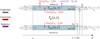 |
Fig. 8 Heat transfers seen by the walls. |
4.4 Governing equations
The system of partial differential equations (eq. (Σ1)) derived from energy balances (Eqs. (5), (14), and (15)) has been defined for the reactor domain (Ω2). The upstream (Ω1) and downstream (Ω3) domains are modeled using the same set of equations, except that the plasma power density term p(x) is set to zero.
See equation. (Σ1) below.
 (Σ1)
(Σ1)
The system is solved under the following assumptions and boundary conditions:
Steady-state: The transient gas temperature field cannot be resolved by spectroscopy, as the exposure time (40 s) leads to temporal averaging over a significant fraction of the gas thermal time constant (120 s).
Continuity of the temperature field: The temperature field is continuous across the interfaces Ω1/Ω2 and Ω2/Ω3.
Inlet boundary condition: The gas enters the domain Ω1 at the ambient temperature, i.e., T(0, t) = 293 K.
The model is solved numerically using COMSOL Multiphysics via the Coefficient Form PDE interface, which handles general partial differential equations system of the form:
 (17)
(17)
 (18)
(18)
The matrices da, α, and γ are null.
These matrices (eqs. (28)) are the direct translation of the system (Eq. (Σ1), expressed using the COMSOL formalism.
4.5 Validation
Figure 9 shows the steady-state temperature profile T(x) computed for a typical set of parameters corresponding to our experimental conditions. As expected, the temperature of the outer quartz wall is lower than that of the gas due to convective cooling at the reactor surface. The gas temperature inside the reactor is non-uniform and typically increases from about 300 K at the inlet to approximately 500 K at the outlet. The inner wall is at nearly the same temperature as the gas. The simulation results are computed almost instantly on a standard laptop.
Figure 10 illustrates the influence of the gas flow rate (ranging from 1 to 10 L/min, corresponding to the operating range of our test bench) on the gas temperature profile along the reactor. At low flow rates (e.g., 1 L/min), thermal conduction dominates over convective transport. As a result, the temperature profile exhibits a smooth, rounded shape due to heat diffusion through the quartz walls, which even leads to a slight preheating of the gas before entering the active discharge zone. At higher flow rates, convective transport becomes the prevailing mechanism, and the temperature field evolves toward a first-order exponential profile characteristic of advection-dominated regimes.
To assess the validity of the analytical 1D model, its predictions are compared, in Figure 7, with a 2D axisymmetric finite element model (FEM) of the reactor, implemented in COMSOL Multiphysics. The FEM model incorporates the same physical parameters and assumptions as the analytical model, except that it resolves radial temperature variations within the three material layers (gas, inner quartz wall, and outer quartz wall). The comparison shows that both models predict very similar axial temperature profiles. As expected, the analytical model corresponds closely to the radial average of the FEM temperature field, demonstrating that the simplifying assumption of radial uniformity provides an accurate representation of the overall thermal behavior of the reactor. This validation confirms the reliability of the analytical model while maintaining its computational simplicity. Moreover, it should be outlined here that the proposed model is fully analytical, which allows one to use it to study the impact of each one of its parameters (for system sizing and/or optimization purposes), which is, with a FEM model, only possible through multiple iterations. The radial uniformity assumption is valid for the present reactor configuration, characterized by a relatively small gas gap (1.6 mm) and both quartz walls (1.2 mm). However, this assumption may no longer hold for significantly larger wall thicknesses, as increased thermal resistance in the walls would induce larger radial temperature differences, which in turn alter the gas–wall interface temperature and thereby affect the heat transfer.
The next step is to compare these predictions with experimental measurements, using optical emission spectroscopy for gas temperature and IR thermography for the outer wall. This comparison allows a quantitative validation of the model under various operating conditions.
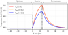 |
Fig. 9 Typical steady-state temperature profile inside the duct. |
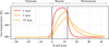 |
Fig. 10 Influence of gas flow rate on the gas temperature profile. |
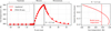 |
Fig. 11 Gas temperature along the reactor: analytical 1D model (solid line) versus radial mean from 2D FEM model (points). The close match shows the analytical model captures the mean thermal behavior accurately. |
5 Results
The following investigations are aimed at validating the simulation results, focusing on the calculated and measured temperatures distributions. Common conditions for the sweeps presented in Section 5. are:
Uniform power dissipation: The operating conditions are selected to promote a uniform discharge regime (according to visual observation), allowing the power density to be reasonably approximated as uniform along the reactor length,  , where Pelec is the mean electrical power injected into the reactor over one period of the power supply.
Thermal steady state conditions.
5.1 Gas temperature as a function of gas flow rate
The purpose of this first experimental campaign is to characterize the gas temperature field inside the reactor as a function of the gas flow rate. The main experimental conditions are as follows:
Electrical operating point: All measurements are obtained at a fixed electrical operating point (
 % corresponding to an injected electrical power of 45 W.
Reactor geometry: The reactor is the 12.5 cm long one (see Fig. 1).
Figure 12 presents the model predictions and the experimentally measured gas temperature profiles for four different flow rates: 0.5, 2, 6, and 10 L/min. This flow-rate sweep covers the entire operating range of the test bench, thereby providing a comprehensive validation of the model under the relevant experimental conditions. The gas temperature is measured by mean of the spectroscopy method introduced in Section 3.1. The five black dots shown in each graph are the five values acquired with five different positions of the collimator along the reactor’s axis. The maximum relative deviation between model predictions and spectroscopic measurements is 19%, observed at the highest flow rate of 10 L/min, while all other operating points remain below 10%. The error bars represent the maximum deviation from the mean value calculated over five measurements performed under identical conditions on five different days over a 4-month period.
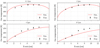 |
Fig. 12 Gas temperature fields as a function of gas flow rate–45 W. The maximum relative deviation between model and measurement is 19%. |
5.2 Gas temperature as a function of electrical power
Building on the previous campaign focused on gas flow rate, this second series of experiments examines the influence of electrical power on the gas temperature. The main experimental conditions are as follows:
Electrical operating point: The injected electrical power is varied in the range 20–50 W by adjusting the discharge current J, while all other operating parameters are kept constant. This power range is chosen to ensure that the reactor reaches thermal steady state without excessive heating (T > 160°C), which could compromise the reactor’s integrity.
Reactor geometry: The reactor length is 7.7 cm, shorter than in the previous campaign, in order to additionally test the robustness of the model with respect to reactor geometry.
Figure 13 presents the model predictions and the experimental gas temperature measured at the middle (x = 3.85 cm) of the reactor for injected powers in the 20–50 W range, at three different gas flow rates (2, 6, and 10 L/min). The maximum relative deviation is 14.5%, at 10 L/min, with deviations way below 10% for all other conditions.
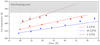 |
Fig. 13 Gas temperature at the middle of the reactor as a function of electrical power and flow rate. The maximum relative deviation between model and measurement is 30%. |
5.3 Outer quartz wall temperature
The purpose of this third experimental campaign is to validate the ability of the model to also predict the outer quartz wall temperature. Measurements are performed using an IR camera, with the experimental protocol detailed in Section 3.2. The main experimental conditions are quite similar to previous ones:
Electrical operating point: The injected electrical power is varied in the range 20–50 W by adjusting the discharge current J, while all other operating parameters are kept constant.
Reactor geometry: The reactor length is 7.7 cm.
Figures 14–16 present the comparison between the model predictions and the experimental outer wall temperature field measured with the IR camera for injected powers in the 20–55 W range, at three different gas flow rates (2, 6, and 10 L/min). The maximum relative deviation between measurements and model reaches 30%, observed at 2 L/min and the highest injected power (Fig. 11), while all other conditions remain way below 10%.
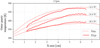 |
Fig. 14 Comparison between the outer quartz wall temperature field measured by IR thermography and the thermal model prediction. Gas flow is 2 L/min. The maximum relative deviation is 30%. |
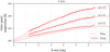 |
Fig. 15 Comparison between the outer quartz wall temperature field measured by IR thermography and the thermal model prediction. |
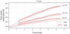 |
Fig. 16 Comparison between the outer quartz wall temperature field measured by IR thermography and the thermal model prediction. |
6 Discussion—–gas temperature distributions open a wide range of system-level investigations
Despite the overall good agreement, some relative deviations remain, notably for the outer wall temperature at low flow rates and high power (Fig. 14) and for the gas temperature at the highest flow rate of 10 L/min (Fig. 12). Several factors may contribute to these discrepancies:
Uniform power dissipation: The model assumes uniform volumetric power deposition in the plasma and neglects possible local non-uniformities that may locally enhance or reduce heating.
Thermal losses: Convective and radiative heat losses to the environment are estimated using simplified coefficients, which may not capture all spatial or temporal variations.
High-flow effects: At 10 L/min, the flow may transition from laminar to partially turbulent, enhancing convective heat transfer beyond what the current model captures.
Measurement uncertainties: Experimental data are affected by limitations of the diagnostic techniques, with spectroscopic gas temperature measurements estimated to have ∼10% error and IR wall temperature measurements ∼13% error.
These limitations explain, at least partially, the observed deviations and highlight potential avenues for future refinement of the model, such as incorporating spatially-resolved plasma power density p(x) [28] or more detailed fluid dynamic modeling for high flow rates.
Beyond its validation against experimental data, the thermal model also provides a powerful framework for analyzing plasma-assisted processes such as NOx removal [29,30]. Because the efficiency of pollutant conversion is highly sensitive to the local gas temperature, accurately predicting the temperature field under various operating conditions is essential for coupling with plasma-chemical kinetics models. This coupling enables a realistic estimation of reaction rates and, so, abatement efficiencies, thereby bridging the gap between purely electrical characterization and comprehensive plasma-chemical simulations.
The influence of the non-uniform temperature field manifests primarily through two mechanisms. First, temperature gradients directly modify the kinetics of plasma-chemical reactions via their Arrhenius dependence, leading to spatially varying reaction rates along the reactor. Second, the non-uniform temperature field induces corresponding variations in gas density along the reactor, according to the ideal gas law at constant pressure. The following sections examine these two coupled effects and their consequences on reaction kinetics, gas flow, and electrical behavior.
-
Direct impact on reaction kinetics: Spatial variations in gas temperature directly affect the reaction kinetics of NOx treatment through the Arrhenius-type dependence of rate coefficients. Consequently, the temperature field Tg(x) translates into a spatially varying set of reaction rates along the reactor axis. Table 2 summarizes the main reactions involved in plasma-assisted NOx conversion, classified according to their role in NO reduction or undesirable oxidation. Most of these reactions (R2–R7) exhibit explicit temperature dependence in their rate constants. As an illustration, the reaction
 (R2) plays a critical role in NO reduction. According to its Arrhenius expression, an increase in gas temperature from 300 to 500 K—typical of our experimental conditions—leads to an increase of approximately 73% in the rate coefficient. These results highlight that even modest temperature gradients along the reactor can cause non-uniform reaction kinetics, potentially shifting the balance between reduction and oxidation pathways. Incorporating the axial temperature field Tg(x) into plasma-kinetic simulations (e.g., with ZdplasKin [31–34]) is therefore essential to accurately predict NOx removal efficiency under realistic operating conditions.
The dissociation reactions (R1) and (R3) are also indirectly influenced by temperature through the gas density N, as discussed in the following section.
-
Indirect impact through gas density variations: At constant atmospheric pressure patm, a non-uniform gas temperature necessarily results in a non-uniform gas density. According to the ideal gas law, the density can be expressed in two ways: (i) as the mass density ρg in kg/m3 (eq. 19) commonly used in thermal and fluid analyses; (ii) as the molecular number density N in m-3 (eq. 20), typically used in plasma physics. Both quantities exhibit the same inverse dependence on gas temperature. Figure 17 illustrates the equation (19) with a typical temperature field.
 (19)
(19) (20)
(20)This non-uniform gas density leads to consequences on other key parameters:
-
Velocity and residence time: At constant mass flow rate and atmospheric pressure, the gas velocity v(x) becomes non-uniform. Indeed, since we are in steady-state, the conservation of mass flow rate ṁ (eq. 21) inside the reactor leads to the expression of gas velocity as a function of temperature (eq. 22):
 (21)
(21) (22)
(22)Figure 15 illustrates the axial variation of gas velocity with the same temperature field as Figure 18. Consequently, the residence time Δtr (eq. 23), a key parameter for the treatment, depends not only on the imposed gas flow rate but also on the injected power and the reactor geometry, through the gas temperature:
 (23)
(23)In the literature, the residence time is commonly estimated as the ratio between the reactor volume and the volumetric gas flow rate. This definition implicitly assumes a constant volumetric flow rate along the reactor. In our study, this assumption is not valid due to the significant spatial variations of the gas temperature, which lead to local variations of the gas density. Therefore, the residence time must be evaluated using the local gas velocity, as expressed in equation (23).
Reduced electric field: Spatial variations of density N(x) lead to spatial variations of the reduced electric field, expressed as E/N(x), which strongly influence the dissociation rates of N2 (Tab. 2, reaction R1) and O2 (Tab. 1, reaction R3), and therefore the overall efficiency of NOx removal.
These coupled effects demonstrate that the thermal model provides critical input to plasma-kinetic solvers such as ZdplasKin. It enables consistent evaluation of how gas flow rate, injected power, and reactor geometry jointly influence the efficiency and stability of plasma-based NOx treatment.
Main reactions, with their rate coefficient, involved in NOx treatment.
7 Conclusion
A parametric analytical model is presented: it describes the gas temperature field in a dielectric barrier discharge reactor used for plasma-assisted gas treatment (NOx abatement in our study). The model provides a simple yet physically consistent description of the coupled heat transfer mechanisms within the reactor, accounting for conduction through the quartz walls and convection due to the gas flow. Despite its simplicity, the analytical formulation enables a fast evaluation of the temperature field—each simulation run requires less than a second—which makes it particularly suitable for parametric studies and coupling with plasma-chemical solvers.
Model predictions are compared to a 2D axisymmetric FEM simulation (COMSOL) and to experimental measurements obtained by IR thermography and optical emission spectroscopy. The analytical and FEM models exhibit very similar profiles, the analytical solution corresponding to the mean radial temperature extracted from the FEM results. Experimental validation confirms the overall reliability of the model, with deviations generally within 10%–15% of measured values.
Beyond this validation, the thermal model is used to analyze how spatial temperature variations influence, on the first hand, gas flow behavior (speed distribution) and key plasma parameters such as gas density, which are not simply controlled by the mass flow controllers; and on the second hand, kinetic mechanisms though variation of the reaction rates and residence time. These effects demonstrate the strong thermal–electrical coupling that governs pollutant conversion efficiency and highlight the interest of the proposed model.
Glossary
DBD: Dielectric barrier discharge
NTP: Non-thermal plasma
MFC: Mass flow controller
Acknowledgments
The authors are deeply grateful to E. BRU who made the “deNOx” test bench possible.
Funding
This research received no external funding.
Conflicts of interest
The authors have nothing to disclose.
Data availability statement
This article has no associated data generated.
Author contribution statement
All authors contributed to the deductions of this study. The development of the thermal model was carried out by N.B., with all authors contributing to its validation. The initial draft of this manuscript was written by N.B. and H.P., with N.M. providing comments on earlier versions. All authors have read and approved the final version.
References
- J.Q. Koenig, Health Effects of Nitrogen Dioxide, in Health Effects of Ambient Air Pollution: How Safe Is the Air We Breathe? (Springer US, Boston, MA, 2000) p. 165. https://doi.org/10.1007/978-1-4615-4569-9_12 [Google Scholar]
- A. Chaloulakou, I. Mavroidis, I. Gavriil, Compliance with the annual NO₂ air quality standard in Athens. Required NOx levels and expected health implications, Atmos. Environ. 42, 454 (2008). https://doi.org/10.1016/j.atmosenv.2007.09.067 [Google Scholar]
- S. Devahasdin, C. Fan, K. Li, D.H. Chen, TiO₂ photocatalytic oxidation of nitric oxide: Transient behavior and reaction kinetics, J. Photochem. Photobiol. A: Chem. 156, 161 (2003). https://doi.org/10.1016/S1010-6030(03)00005-4 [Google Scholar]
- W.S. Tunnicliffe, P.S. Burge, J.G. Ayres, Effect of domestic concentrations of nitrogen dioxide on airway responses to inhaled allergen in asthmatic patients, Lancet 344, 1733 (1994). https://doi.org/10.1016/S0140-6736(94)92886-X [Google Scholar]
- K. Skalska, J.S. Miller, S. Ledakowicz, Trends in NOx abatement: A review, Sci. Total Environ. 408, 3976 (2010). https://doi.org/10.1016/j.scitotenv.2010.06.001 [Google Scholar]
- L. Alves et al., A comprehensive review of NOx and N₂O mitigation from industrial streams, Renew. Sustain. Energy Rev. 155, 111916 (2022). https://doi.org/10.1016/j.rser.2021.111916 [Google Scholar]
- P. Talebizadeh, M. Babaie, R. Brown, H. Rahimzadeh, Z. Ristovski, M. Arai, The role of non-thermal plasma technique in NOx treatment: a review, Renew. Sustain. Energy Rev. 40, 886 (2014). https://doi.org/10.1016/j.rser.2014.07.194 [Google Scholar]
- N.V.R. Rueda, Reduction of nitrogen oxides in diesel exhaust using dielectric barrier discharges driven by current-mode power supplies, PhD thesis, Institut National Polytechnique de Toulouse, Toulouse, 2022. https://theses.hal.science/tel-04248330 [Google Scholar]
- W. Zhang et al., Experimental and mechanism research on the NOx removal by a novel liquid electrode dielectric barrier discharge reactor, Chem. Eng. J. 443, 136375 (2022). https://doi.org/10.1016/j.cej.2022.136375 [Google Scholar]
- S. Mohapatro, S. Allamsetty, A. Madhukar, N.K. Sharma, Nanosecond pulse discharge based nitrogen oxides treatment using different electrode configurations, High Volt. 2, 121 (2017). https://doi.org/10.1049/hve.2017.0011 [Google Scholar]
- C.R. McLarnon, B.M. Penetrante, Effect of reactor design on the plasma treatment of NOx, in International Fall Fuels and Lubricants Meeting and Exposition (San Francisco, California, United States, October 19, 1998). https://doi.org/10.4271/982434 [Google Scholar]
- T. Wang et al., Effect of reactor structure in DBD for nonthermal plasma processing of NO in N2 at ambient temperature, Plasma Chem. Plasma Process. 32, 1227 (2012). https://doi.org/10.1007/s11090-012-9399-3 [Google Scholar]
- R.M. Renneke, L.A. Rosocha, Y. Kim, Temperature effects on gaseous fuel cracking studies using a dielectric barrier discharge, IEEE Trans. Plasma Sci. 36, 3091 (2008). https://doi.org/10.1109/TPS.2008.2003193 [Google Scholar]
- T. Wang, B. Sun, Effect of temperature and relative humidity on NOx removal by dielectric barrier discharge with acetylene, Fuel Process. Technol. 144, 109 (2016). https://doi.org/10.1016/j.fuproc.2015.12.027 [Google Scholar]
- A.-M. Zhu, Q. Sun, J.-H. Niu, Y. Xu, Z.-M. Song, Conversion of NO in NO/N2, NO/O2/N2, NO/C2H4/N2 and NO/C2H4/O2/N2 systems by dielectric barrier discharge plasmas, Plasma Chem. Plasma Process. 25, 313 (2005). https://doi.org/10.1007/s11090-004-3134-7 [Google Scholar]
- P. Talebizadeh et al., Evaluation of residence time on nitrogen oxides removal in non-thermal plasma reactor, PLoS One 10, e0140897 (2015). https://doi.org/10.1371/journal.pone.0140897 [Google Scholar]
- S.J. Anaghizi, P. Talebizadeh, H. Rahimzadeh, H. Ghomi, The configuration effects of electrode on the performance of dielectric barrier discharge reactor for NOx removal, IEEE Trans. Plasma Sci. 43, 1854 (2015). https://doi.org/10.1109/TPS.2015.2422779 [Google Scholar]
- P. Talebizadeh, H. Rahimzadeh, S.J. Anaghizi, H. Ghomi, M. Babaie, R.J. Brown, Experimental study on the optimization of dielectric barrier discharge reactor for NOx treatment, IEEE Trans. Dielectr. Electr. Insul. 23, 3872 (2016). https://doi.org/10.1109/TDEI.2016.005690 [Google Scholar]
- N. Dubus, Contribution à l’étude thermique d’un réacteur à décharge à barrière diélectrique, PhD thesis, Université de Poitiers, Poitiers, 2009. https://theses.fr/2009POIT2318 [Google Scholar]
- H. Sadat, N. Dubus, L. Pinard, J.M. Tatibouet, J. Barrault, Conduction heat transfer in a cylindrical dielectric barrier discharge reactor, Appl. Therm. Eng. 29, 1813 (2009). https://doi.org/10.1016/j.applthermaleng.2008.06.006 [Google Scholar]
- B. Jayaraman, W. Shyy, Modeling of dielectric barrier discharge-induced fluid dynamics and heat transfer, Prog. Aerosp. Sci. 44, 139 (2008). https://doi.org/10.1016/j.paerosci.2007.10.004 [Google Scholar]
- N. Bente, Étude système d’un dispositif de décharges à barrières diélectriques dédié à la réduction des oxydes d’azote, PhD thesis, Université de Toulouse, 2025. Accessed on 19 September 2025. https://theses.fr/2025TLSEP026 [Google Scholar]
- W.M. Rohsenow, J.P. Hartnett, Y.I. Cho (Eds.), Handbook of heat transfer, 3rd ed. (McGraw-Hill, New York, 1998) [Google Scholar]
- D. Florez, R. Diez, H. Piquet, A.K.H. Harb, Square-shape current-mode supply for parametric control of the DBD excilamp power, IEEE Trans. Ind. Electron. 62, 1451 (2015). https://doi.org/10.1109/tie.2014.2361601 [Google Scholar]
- D.M. Florez Rubio, Power supplies for the study and efficient use of DBD excimer UV lamps, PhD thesis, Institut National Polytechnique de Toulouse, Toulouse, 2014. https://www.theses.fr/2014INPT0003 [Google Scholar]
- N. Britun, M. Gaillard, A. Ricard, Y.M. Kim, K.S. Kim, J.G. Han, Determination of the vibrational, rotational and electron temperatures in N2 and Ar–N2 RF discharge, J. Phys. D Appl. Phys. 40, 1022 (2007). https://doi.org/10.1088/0022-3727/40/4/016 [Google Scholar]
- B.M. Penetrante, M.C. Hsiao, B.T. Merritt, G.E. Vogtlin, Fundamental limits on NOx reduction by plasma, SAE Technical Paper 971715 (1997). https://doi.org/10.4271/971715 [Google Scholar]
- V. Rueda, R. Diez, N. Bente, H. Piquet, Combined image processing and equivalent circuit approach for the diagnostic of atmospheric pressure DBD, Appl. Sci. 12, 8009 (2022). https://doi.org/10.3390/app12168009 [Google Scholar]
- N. Bente, A. Cuellar Valencia, H. Piquet, Minimization of chemical kinetic reaction set for system-level study of non-thermal plasma NOx abatement process, Plasma 8, 36 (2025). https://doi.org/10.3390/plasma8030036 [Google Scholar]
- L. Pitchford et al., LXCat: an open-access, web-based platform for data needed for modeling low temperature plasmas, Plasma Process. Polym. 14, 1600098 (2017) [Google Scholar]
- S. Pancheshnyi, B. Eismann, G.J.M. Hagelaar, L.C. Pitchford, Computer code ZDPlasKin, University of Toulouse, CNRS-UPS-INP, Toulouse, France, 2008. http://www.zdplaskin.laplace.univ-tlse.fr [Google Scholar]
- G.J.M. Hagelaar, L.C. Pitchford, Solving the Boltzmann equation to obtain electron transport coefficients and rate coefficients for fluid models, Plasma Sources Sci. Technol. 14, 722 (2005). https://doi.org/10.1088/0963-0252/14/4/011 [Google Scholar]
- S. Pancheshnyi et al., The LXCat project: electron scattering cross sections and swarm parameters for low temperature plasma modeling, Chem. Phys. 398, 148 (2012). https://doi.org/10.1016/j.chemphys.2011.04.020 [NASA ADS] [CrossRef] [Google Scholar]
- E. Carbone et al., Data needs for modeling low-temperature non-equilibrium plasmas: the LXCat project, history, perspectives and a tutorial, Atoms 9, 16 (2021). https://doi.org/10.3390/atoms9010016 [Google Scholar]
- B.M. Penetrante et al., Pulsed corona and dielectric-barrier discharge processing of NO in N2, Appl. Phys. Lett. 68, 3719 (1996). https://doi.org/10.1063/1.115984 [Google Scholar]
- M.A.A. Clyne, I.S. McDermid, Mass spectrometric determinations of the rates of elementary reactions of NO and NO2 with ground state N(4S) atoms, J. Chem. Soc. Faraday Trans. 171, 2189 (1975). https://doi.org/10.1039/F19757102189 [Google Scholar]
- W. Tsang, J.T. Herron, Chemical kinetic data base for propellant combustion I. reactions involving NO, NO2, HNO, HNO2, HCN and N2O, J. Phys. Chem. Ref. Data 20, 609 (1991). https://srd.nist.gov/JPCRD/jpcrd417.pdf [Google Scholar]
- R. Atkinson, D.L. Baulch, R.A. Cox, R.F. Hampson Jr., J.A. Kerr, J. Troe, Evaluated kinetic and photochemical data for atmospheric chemistry: supplement IV. IUPAC subcommittee on gas kinetic data evaluation for atmospheric chemistry, J. Phys. Chem. Ref. Data 21, 1125 (1992). https://doi.org/10.1063/1.555918 [Google Scholar]
Cite this article as: Nicolas Bente, Hubert Piquet, Nofel Merbahi, Analytical thermal model for cylindrical DBD reactors: how to obtain a reliable gas temperature distribution, and why is it so important, Eur. Phys. J. Appl. Phys. 101, 12 (2026), https://doi.org/10.1051/epjap/2026008
All Tables
All Figures
|
Fig. 1 Overview of the “deNOx” test bench. |
| In the text | |
|
Fig. 2 Gas temperature measurement setup. |
| In the text | |
|
Fig. 3 Typical measured spectrum around 774 nm. |
| In the text | |
|
Fig. 4 Transversal view of the reactor, taken by the FLIR E75 thermal camera. |
| In the text | |
|
Fig. 5 Corresponding thermogram of the reactorsurface recorded at thermal steady state. |
| In the text | |
|
Fig. 6 Schematic of the reactor. |
| In the text | |
|
Fig. 7 Elementary slices of the annular duct. |
| In the text | |
|
Fig. 8 Heat transfers seen by the walls. |
| In the text | |
|
Fig. 9 Typical steady-state temperature profile inside the duct. |
| In the text | |
|
Fig. 10 Influence of gas flow rate on the gas temperature profile. |
| In the text | |
|
Fig. 11 Gas temperature along the reactor: analytical 1D model (solid line) versus radial mean from 2D FEM model (points). The close match shows the analytical model captures the mean thermal behavior accurately. |
| In the text | |
|
Fig. 12 Gas temperature fields as a function of gas flow rate–45 W. The maximum relative deviation between model and measurement is 19%. |
| In the text | |
|
Fig. 13 Gas temperature at the middle of the reactor as a function of electrical power and flow rate. The maximum relative deviation between model and measurement is 30%. |
| In the text | |
|
Fig. 14 Comparison between the outer quartz wall temperature field measured by IR thermography and the thermal model prediction. Gas flow is 2 L/min. The maximum relative deviation is 30%. |
| In the text | |
|
Fig. 15 Comparison between the outer quartz wall temperature field measured by IR thermography and the thermal model prediction. |
| In the text | |
|
Fig. 16 Comparison between the outer quartz wall temperature field measured by IR thermography and the thermal model prediction. |
| In the text | |
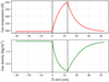 |
Fig. 17 Axial variation of gas density (eq. 19) for a typical gas temperature field. |
| In the text | |
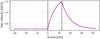 |
Fig. 18 Axial variation of gas velocity (eq. 22) for a typical gas temperature field. |
| In the text | |
Current usage metrics show cumulative count of Article Views (full-text article views including HTML views, PDF and ePub downloads, according to the available data) and Abstracts Views on Vision4Press platform.
Data correspond to usage on the plateform after 2015. The current usage metrics is available 48-96 hours after online publication and is updated daily on week days.
Initial download of the metrics may take a while.