| Issue |
Eur. Phys. J. Appl. Phys.
Volume 100, 2025
Special Issue on ‘Electromagnetic modeling: from material properties to energy systems (Numelec 2024)’, edited by Lionel Pichon and Junwu Tao
|
|
|---|---|---|
| Article Number | 22 | |
| Number of page(s) | 9 | |
| DOI | https://doi.org/10.1051/epjap/2025020 | |
| Published online | 25 August 2025 | |
https://doi.org/10.1051/epjap/2025020
Original Article
Application of HBM and POD for insulation assessment of oil-paper insulation system with nonlinear properties
1
State Key Laboratory of Power Transmission Equipment and System Security and New Technology, 400044 Chongqing, China
2
Group of Electrical and Electronic Engineering of Paris, Sorbonne Université, CNRS, 75005 Paris, France
3
Group of Electrical and Electronic Engineering of Paris, Université Paris-Saclay, CentraleSupélec, CNRS, 91190 Paris, France
* e-mail: This email address is being protected from spambots. You need JavaScript enabled to view it.
Received:
21
September
2024
Accepted:
9
July
2025
Published online: 25 August 2025
Abstract
The oil-paper insulation system of converter transformers operates under periodic composite AC & DC voltages, with its insulation ability determined by permittivity and conductivity. In the assessment of insulation state, the harmonic balance method (HBM) is adopted in electro-quasi-static field problems to consider the harmonic dependence of permittivity. To reduce the computational burden, proper orthogonal decomposition (POD) is incorporated into the HBM scheme to decrease computational complexity, and a sampling method is put forward based on the characteristics of power system harmonics. Additionally, the nonlinear electric field dependence of the conductivity of the oil-paper insulation system is taken into account in the insulation assessment, which is addressed using the fixed-point iteration method in this paper. Finally, a model of a converter transformer is constructed to demonstrate the effectiveness of the HBM-POD approach.
Key words: Hamonic balance method / model order reduction / nonlinear system / oil-paper insulation / periodic problems
© C. Chi et al., Published by EDP Sciences, 2025
 This is an Open Access article distributed under the terms of the Creative Commons Attribution License (https://creativecommons.org/licenses/by/4.0) which permits unrestricted use, distribution, and reproduction in any medium, provided the original work is properly cited.
1 Introduction
Converter transformers, unlike traditional AC power transformers, connect AC systems to a DC link. In the high voltage direct current (HVDC) systems, on the one side, converter transformers link the AC network on its input side and supply stable DC power to the DC link on its output side, functioning as a rectifier; on the opposite side, converter transformers connect to the DC link on its input side and deliver AC power to the AC network, operating as an inverter [1], as shown in Figure 1a. Clearly, serving as barriers between AC systems and the DC link, converter transformers withstand composite AC & DC voltages. The grid-side bushing of converter transformers is connected to the AC network, while the valve-side bushing is connected to the converter valve, subject to a composite voltage, as shown in Figure 1b. Inside converter transformers, the transformer oil together with the paper components, including the ring angle, spacers, and insulation layer, constitutes the oil-paper insulation system. This system would withstand periodic composite AC & DC voltage excitations.
To study the main components of composite voltages, a previous study [2] built a simulation circuit for HVDC, including a converter transformer, converter valves, and smoothing reactors, to imitate actual operating conditions and obtain the voltage data. A frequency spectrum analysis reveals that the periodic voltage excitation consists of a DC component, a fundamental AC component, and higher-order harmonics. It is clear that the DC, fundemental AC and lower-order harmonics dominate the composite voltage excitation, while the magnitude of the voltage decreases progressively with increasing harmonic order. Besides, this composite voltage excitation causes the oil-paper insulation system to experience a special insulation state: when subjected to a DC voltage, the insulation status of the oil-paper insulation system experiences a resistive effect, whereas under the fundamental AC voltage and harmonic components, it experiences in addition a capacitive effect. Consequently, the insulation capability is determined by both permittivity and conductivity. Moreover, these physical properties are influenced by various factors, such as temperature, moisture, and pressure. Experiments indicates that the permittivity of paper decreases with an increase in harmonic order [3], and its conductivity shows a nonlinear dependence on electric field intensity [4].
However, there are currently no efficient approaches that consider the physical properties of the oil-paper insulation system in insulation assessments, in which the permittivities of transformer oil and paper depend on frequency, and the conductivities depend on electric field intensity. Earlier studies estimated the insulation status under composite voltages in the time domain [5], however, this method requires iterating through thousands of cycles to reach a periodic steady state due to the large time constant, on the order of several thousand seconds, caused by the low conductivity of the oil-paper insulation system [6]. Additionally, one cycle in the power system is equivalent to 0.02 s, and it can be deduced that more than one hundred thousand cycles would need to be computed to reach the steady state. Until HBM was proposed and applied to electromagnetic analysis, thereby simplifying the calculation of periodic multiple harmonics. But this approach [7] generates a large coefficient matrix due to the involvement of various harmonics, imposing a significant computational burden. Additionally, the computation for the nonlinear dependence of conductivity is iterative [8], necessitating to update all degrees of freedoms (DoFs) of the unknown variables in each iteration. Moreover, the large size and detailed components of converter transformer models result in a higher number of finite elements' DoFs in modeling, further increasing computational complexity.
In this paper, we propose a model order reduction method based on the HBM-POD approach to study the insulation status of the oil-paper insulation system under composite AC & DC voltages. This method utilizes the HBM to account for the frequency dependence of permittivity and employs fixed-point iteration to address the electric field dependence of conductivity. Additionally, POD is introduced into the HBM scheme to reduce computational cost in the harmonic domain, and a sampling method is provided based on the characteristic of power system harmonics that the DC, fundemental AC and lower-order components dominate the composite voltage excitation.
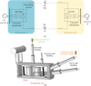 |
Fig. 1 Topology diagram of HVDC system (a), and converter transformer structure (b). |
2 EQS field problem of oil-paper insulation
Under rated conditions, the composite voltage excitation experienced by converter transformers is considered as a low-frequency signal, and the oil-paper insulation system is regarded as a poor conductor, where the magnitudes of conduction current density and displacement current density are comparable. Additionally, the induced electric field strength caused by magnetic field variations is negligible. Therefore, the insulation state of the oil-paper insulation system is classified as an electro-quasi-static field [9], as given
 (1)
(1)
where φ is the electric potential, ϵ is the permittivity dependent on the frequency, γ is the conductivity nonlinearly dependent on the electric field, u (t) is the composite AC & DC voltage excitations. Ω is the research domain, and Γ1 and Γ2 are such that ∂Ω = Γ1 ∪ Γ2, where ∂Ω is the boundary of Ω.
By using the finite element method to discretize the solution domain in space, a semi-discrete form of the equation is obtained as
 (2)
(2)
where Kγ (φ) is a conductivity coefficient matrix that requires updating based on the electric field, and Kϵ is a permittivity coefficient matrix dependent on the frequency.
3 Model order reduction approach
The oil-paper insulation system with nonlinear properties will be studied for its insulation capability using an effective method. HBM is employed to analyze the frequency-dependent properties of permittivity, while the fixed-point iteration method is used to examine the nonlinear electric-field-dependent properties of conductivity. Additionally, to reduce computational cost, POD is led into HBM based on sampling in the harmonic domain, thereby reducing the number of unknowns for the electric potential variable. Moreover, this approach provides a way to determine orthogonal bases for each harmonic order, taking into account HVDC operating conditions in which the magnitudes of certain harmonics are significant while others can be neglected.
3.1 Harmonic balance method for EQS field
To consider the frequency dependence of permittivity, the assessment computation of insulation ability would be studied in the harmonic domain. The electric potential is expanded in harmonic domain as a complex Fourier series. Since the voltage excitation signal is a real-valued signal, only half of harmonic coefficient would be computed, and all harmonic coefficient would be obtained by the conjugate symmetry [10]. The complex Fourier series with positive indices is given by (3).
 (3)
(3)
where  , 𝒩 is the order of the truncated harmonics, φ𝒽 is the 𝒽-th harmonic component and φ0 is the DC component.
The electric potential in the time domain could be represented in the harmonic domain, as  where a𝒽 is a column vector of size Ns and Ns is the number of DoFs for the discretization in space.
 (4)
(4)
where hH (t) is a row matrix consisting of exponential function, as hH (t) = [e0, ejωt, … , ej𝒽ωt, … , ej𝒩ωt], E is an Ns × Ns identity matrix, and φ (t) is the matrix format of electric potential in time domain.
Meanwhile,  could also be represented by φH, so a differential matrix ε is introduced to handle (4) and is defined by a diagonal matrix ε = diag (0, jω, … , j𝒽ω, … , j𝒩ω) [11]:
 (5)
(5)
Substituting (4) and (5) into (2) yields
 (6)
(6)
Multiplying (6) by each component  of hH, integrating over one cycle T yields, and then dividing by T yields (7):
 (7)
(7)
where  is the 𝒽-th component of hH (t). Besides, based on
  , we have
  , hence the EQS equation, considering the effects of multiple harmonics, is derived using the HBM as (9). It should be noted that although the conductivity coefficient matrix Kγ (φ) generally depends on time-varying electric fields, as will be explained in Section 3.4, when using the fixed point to solve the nonlinear equation, Kγ (φ) is divided into a constant part Kγ,FP and a nonlinear part Kγ,NL, only the constant is considered in the time integration process while the nonlinear part will be put in the right hand side. Under this treatment, considering only the constant part of Kγ (φ), the time integration of (7) leads to
 (8)
(8)
where H (ω) = diag (Kγ, Kγ,FP + jωKϵ,1, … , Kγ,FP + jω𝒽Kϵ,𝓀, … , Kγ,FP + j𝒩ωKϵ,𝒩) in size of Ns (𝒩 + 1) × Ns (𝒩 + 1). Kϵ,𝒽 is the permittivity matrix calculated by the permittivity corresponding to the frequency at  ,F𝒽 is the nonlinear part which will be specified in Section 3.4.
Therefore, for a specific harmonic, such as the 𝒽-th order harmonic, the EQS problem can be expressed as (9) after incorporating the corresponding boundary conditions:
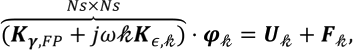 (9)
(9)
where φ𝒽 is the electric potential under the 𝒽-th harmonic and is a column matrix of Ns entries, U𝒽 is the Dirichlet boundary condition in the spatially discretized format, corresponding to u𝒽 after performing a Fourier transform of u (t). For the Dirichlet boundary conditions, the penalty function method is adopted. The treatment of the R.H.S and the coefficient matrix follows the approach described in [12]. Finally, it should be noted that, after incorporating the boundary conditions, the DoF in (9) remains equal to Ns.
3.2 Sampling in harmonic domain
To reduce computational cost, electric potential information is collected as samples to provide orthogonal basis vectors for the subsequent POD computation. Unlike traditional POD approaches that sample snapshots through time marching, the HBM-POD approach collects samples in the harmonic domain. When constructing a low order subspace for 𝒽-th order harmonic computation, it is essential to formulate a sampling marix consisting of the electric potential at the 𝒽-th order harmonic, expressed as A𝒽 = [φ𝒽,1, φ𝒽,2 … φ𝒽,Nm]. The sampling process begins with conductivity determined under nonlinear DC excitation, which serves as the initial condition for fundamental AC computation in the frequency domain, accounting for nonlinear effects. By applying different fundamental AC voltage excitations, the corresponding electric potential vectors are obtained. Thus, Nm voltage excitations are required to construct a sampling matrix, where Nm represents the reduced DoFs in the subspace, corresponding to the number of unknowns in the reduced-order model. Similarly, electric potentials for other harmonic orders are computed. In this study, only harmonics with large magnitudes are assigned individual orthogonal bases from frequency domain analysis, while low-magnitude harmonics share the basis of their adjacent dominant harmonic.
Performing singular value decomposition on the sampling matrix A𝒽 = [φ𝒽,1, φ𝒽,2 … φ𝒽,Nm] yields a set of orthogonal basis vectors, which can be used to approximate the unknown variable φ𝒽 [13,14], given as
 (10)
(10)
where P𝒽 is a Ns × Nm matrix with Nm orthogonal basis vectors, and V is an orthonormal matrix . Diag (λ1, λ2, … λNm) contains Nm singular values, usually Nm << Ns.
Therefore, the unknown variable φ𝒽 is approximated by
 (11)
(11)
where α𝒽 = [α1, … αNm] T, indicating that α𝒽 with fewer DoFs will replace φ𝒽 as column matrix to be solved in (9).
3.3 HBM-POD scheme
Based on (12), the unknown variable φ𝒽 in HBM is replaced by P𝒽α𝒽, and then P𝒽H (the conjugate transpose of P𝒽.) is multiplied to both sides of (9). The governing equation of HBM-POD scheme is derived, as (13). The coefficient matrix P𝒽H(Kγ + jω𝓀Kϵ,𝒽)P𝒽 is in the size of Nm × Nm, and the number of unknowns decreases from Ns to Nm.
 (12)
(12)
The HBM-POD model computes based on the order number 𝒽. It begins with 𝒽 =0, where the DC component of the voltage excitation is computed first, followed by the fundamental AC voltage component, then the second harmonic, third, fourth, and so on. Each order harmonic has corresponding orthogonal basis.
3.4 Fixed-point iteration
The fixed-point iteration method is utilized to deal with the electric field-dependence of the conductivity, by dividing the nonlinear conductivity into two parts as γFP and γNL. γFP is a fixed-point conductivity, while γNL is a function of electric field and conductivity, that is to say, γ = γFP + γNL. The iterative form is given:
 (13)
(13)
where m is the iteration number; Kγ,FP is the coefficient matrix of fixed-point conductivity γFP, and F𝒽 equals the corresponding 𝒽-th column of −Kγ,NL ⋅ φ (t) (m) after the fast Fourier transform.
Using the fixed-point iteration method, if a fixed conductivity value is maintained throughout the computation, the convergence rate of the system is often unsatisfactory [15]. The error between successive iterations may increase as the number of iterations grows, and the computation may fail to converge. In this paper, the conductivity is updated in each iteration based on the results of the previous iteration [16]:
 (14)
(14)
where  is a fixed-point conductivity at the (m + 1)-th iteration; maxt∈[0,T] (γ (m)) and mint∈[0,T] (γ (m)) are the maximum conductivity and the minimum conductivity of one material at the m-th iteration.
Regarding the convergence of this nonlinear system, the computation ends when the error between the results of two consecutive iterations is less than the specified error tolerance χ:
 (15)
(15)
Moreover, it is worth noting that since the composite AC & DC voltages are real-valued excitations, so the results of electric potential over one period can be obtained by the conjugate symmetry [17], and then be transformed back to the time domain by the inverse Fast Fourier Transform (iFFT).
4 Algorithm
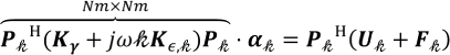
Figure 2 illustrates the computation process. To efficiently consider the frequency dependence of permittivity and the electric field dependence of conductivity, a model order reduction approach to apply POD in HBM is proposed for evaluating the insulation state of the oil-paper system in converter transformers. This model order reduction approach is consisted of two stages: the first stage involves generating samples as a pre-calculation step (highlighted in yellow background), while the second stage is a process based on this model order reduction approach (highlighted in green background).
In the first stage, the full-order model is solved to provide harmonic-domain samples. After determining the reduced order number Nm, the 𝒽-th harmonic order is solved Nm times as described in Section 3.2. This results in a set of electric potential samples denoted as [φ𝒽,1, φ𝒽,2 … φ𝒽,Nm]. Singular value decomposition is then applied to this sampling matrix, yielding an orthogonal basis to approximate the unknown variable. To reduce computational cost in insulation assessment for HVDC systems, harmonics with larger magnitudes are assigned their own orthogonal bases as computed above, while those with smaller magnitudes share the orthogonal basis of an adjacent dominant harmonic.
In the second stage, the model order reduction process begins, where the order is reduced using POD within the HBM scheme. In this approach, when solving for the 𝒽-th harmonic order, the unknown variable is projected onto the corresponding orthogonal basis as (12), and then solved in the reduced-order framework. Once all harmonics are solved, time-domain results are after applying conjugate symmetry and iFFT. Next, an error criterion is then applied to determine whether the nonlinear properties need updating. Notably, the conductivity is updated in the full-order model, hence, before applying conjugate symmetry, the electric potential is transformed to the full order scheme. As shown in Figure 2, only the processes within the dashed frame correspond to the reduced-order model, while all processes within the solid frame belong to the full-order model.
 |
Fig. 2 Flowchart of HBM-POD scheme. |
5 Results and discussion
To validate the proposed HBM-POD approach, a ±500 kV converter transformer model is constructed to study the insulation state of the oil-paper insulation system, taking into account the frequency dependence of permittivity and the electric field dependence of conductivity.
5.1 Model description
A 2D converter transformer model is constructed with a detailed oil-paper insulation system. As shown in Figure 3, the white area represents the transformer tank filling with transformer oil, while the green area represents the transformer paper, which includes the pressboard, angle ring, and insulation layer. After the meshing process, the model has been generated with 79929 nodes and 153692 elements. In the HBM-POD scheme, the order has been reduced to Nm = 5.
The grid winding is marked in red and is connected to a sinusoidal voltage under rated conditions. Meanwhile, the valve winding, marked in blue, is connected to composite AC & DC voltages, as Figure 3. The tank wall is grounded throughout the simulation, and the bottom line of this model represents the symmetric plane with Neumann boundary condition. In this case, the voltage excitations for both windings are shown in Figure 4, and six kinds of sources are consisted of voltage excitation in the system. In this example, only the fundamental AC component and one harmonic order with larger magnitudes have their own corresponding bases, while the other harmonics share the basis of their nearest dominant harmonic. The DC component is not included in the reduced-order computation.
The physical parameters of the oil-paper insulation system are shown in Figure 5. Figure 5a illustrates that the relative permittivity of paper decreases with increasing harmonic order. When the harmonic order is one, the relative permittivity of paper is 5.6; when the harmonic order increases to 49, the relative permittivity decreases to 4.3. Since the change in the relative permittivity of oil with harmonics is not significant in this range, it is set to a constant value of 2.2. Additionally, the nonlinear electric field dependence of conductivity is shown in Figure 5b. The oil's conductivity changes with the electric field in a U-shaped pattern, while the paper's conductivity exhibits exponential growth with increasing electric field.
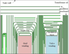 |
Fig. 3 Model of oil-paper insulation system in a converter transformer. |
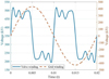 |
Fig. 4 Voltage excitation of valve winding and grid winding. |
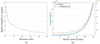 |
Fig. 5 Physical parameters of oil-paper insulation system. |
5.2 Results of HBM-POD approach
Based on the combined approach of HBM-POD, the variation of the electric field over one cycle is computed. As illustrated in Figure 6, the electric potential contours are shown at both a quarter of the cycle and half a cycle. In Figure 6a, the grid-side winding experiences a peak-value sine-wave voltage at this moment, while the valve-side experiences positive composite voltages. It is evident that the equipotential lines near the valve winding are more convoluted, whereas those near the grid winding are smoother. The reason is that near the grid side, the insulation status is capacitive due to the sinusoidal excitation, leading to the oil withstanding a greater electric field as a result of its lower permittivity. In contrast, near the valve winding, the insulation status is more resistive due to the excitation containing a DC component, causing the paper to withstand a greater electric field due to its lower conductivity. Similarly, when the excitation of the grid-winding decreases to zero at the half cycle while the valve-side still experiences positive composite voltages (as Fig. 6b), it can be observed that the equipotential lines in the paper become more convoluted. This indicates that the paper is subjected to a higher electric field.
To study the insulation status of transformer oil, three sampling points were selected: one at the end of the grid winding, another between the two windings, and the third one at the end of the valve winding. These points are used to record the variation in the electric field, as illustrated in Figure 7. It can be observed that the electric field variation in Figure 7a resembles a sine wave, like the voltage excitation of the grid winding. Meanwhile, the electric field trend in Figure 7c follows the voltage excitation of the valve winding. At the point located between the two windings (Fig. 7b), the electric field trend is a combination of the two excitations. This changing process aligns with our expectations.
To check the accuracy of the HBM-POD, the simulation results by HBM-POD are compared with the simulation results of HBM. As shown in Figure 7, the tendency curves of the two approaches almost overlap, indicating that the results of the HBM-POD approach approximate those of the full-order HBM. The maximum relative errors at the three points are 0.5 × 10⁻², 2.4 × 10⁻² and 0.8 × 10⁻² respectively. Notably, all maximum errors occur when the sinusoidal voltage crosses zero. It clear that the HBM-POD maintains higher accuracy.
Additionally, by HBM-POD method, the computational efficiency increases dramatically. All algorithms in the paper were implemented in MATLAB, using an AMD Ryzen 7 6800H processor with 15 GB of RAM. The full-order model by HBM takes 5990 s to reach steady state, while the reduced-order model by HBM-POD takes 701 s in total. It is clear that the computation time is reduced to 11.7% by HBM-POD. Additionally, the sampling process requires a total of 29.1 seconds for Nm snapshots of each voltage component, including a DC component, a fundamental AC component, and four harmonics.
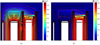 |
Fig. 6 Electric potential distribution at |


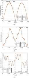 |
Fig. 7 Electric field variation of one cycle at the end of grid winding (a), between two windings (b), and at the end of valve winding (c). |
6 Conclusion
In this paper, the insulation assessment of the oil-paper insulation system is studied under the condition of composite AC & DC voltage excitations. To reduce computational cost, a model order reduction method based on the HBM-POD approach is developed. The unknown variables in the HBM framework are approximated by POD orthogonal basis generated by sampling in the harmonic domain. Additionally, this method accounts for two factors of the oil-paper insulation system: the frequency dependence of permittivity and the electric field dependence of conductivity. To address the issue of nonlinear conductivity, a fixed-point iteration is introduced into the HBM-POD approach.
Taking the converter transformer model as an example, the insulation state of oil-paper insulation system is studied. The accuracy and efficiency of the HBM-POD approach are verified by comparing with the results of the full-order model.
Funding
This work was supported by the National Key R&D Program of China (grant numbers 2021YFB2401700).
Conflicts of interest
The authors declare no conflicts of interest in relation to this article.
Data availability statement
The datasets generated during and/or analysed during the current study are available from the corresponding author on reasonable request.
Author contribution statement
All authors contributed to the theoretical deductions of this study. The program framework design, code debugging, and data analysis were carried out by all authors. The initial draft of this manuscript was written by Cheng Chi, with Zhuoxiang Ren and Fan Yang providing comments on earlier versions. All authors have read and approved the final version.
References
- W. Zhao, HVDC Engineering Technology (China Electric Power Press), 12 (2011) [Google Scholar]
- S.L. Zhang, Z.R. Peng, Design and analysis of insulation structure of ±800 kV valve side converter transformer bushing, High Voltage Eng. 45, 2048 (2019) [Google Scholar]
- Q.Y. Wang, B.D. Bai, D.Z. Chen et al., Study of insulation material properties subjected to nonlinear AC-DC composite electric field for converter transformer, IEEE Trans. Magn. 55, 1 (2018) [Google Scholar]
- L.J. Yang, Z.D. Cheng, L. Cheng et al, Effects of the charge carrier elimination process on oil conductivity decrease under high electric field intensity, IET Sci. Measur. Technol. 14, 979 (2020) [Google Scholar]
- W.D. Sun, L.J. Yang, F. Zare et al., 3D modeling of an HVDC converter transformer and its application on the electrical field of windings subject to voltage harmonics, Int. J. Electr. Power Energy Syst. 117, 105581 (2019) [Google Scholar]
- C. Chi, Z. Ren, F. Yang, Model order reduction based on space-harmonic separation for nonlinear periodic EQS problem, IEEE Trans. Magn. 60, 1 (2024) [Google Scholar]
- E. Sarrouy, J. Sinou, Non-linear periodic and quasi-periodic vibrations in mechanical systems-on the use of the harmonic balance methods, Adv. Vibrat. Anal. Res. 21, 419 (2011) [Google Scholar]
- J. Li, B.X. Du, H.C. Liang et al., Electrical field distribution in ±600 kV converter transformer bushing core with the application of epoxy resin with nonlinear conductivity, in 2018 IEEE International Conference on High Voltage Engineering and Application (ICHVE), IEEE (2018) [Google Scholar]
- H.A. Haus, J.R. Melche, in Chapter 3: Introduction to electroquasistatics and magnetoquasistatics, Electromagnetic Fields and Energy (Prentice Hall, Englewood Cliffs, 1989), pp. 9. [Google Scholar]
- G. Liu, Z. Jin, X.J. Zhao et al., Analysis of nonlinear electric field of oil-paper insulation under non-sinusoidal voltage by the fixed-point harmonic-balanced decomposition FEM, Int. J. Appl. Electromagn. Mech. 60, 393 (2019) [Google Scholar]
- G. Lee, Y. Park, A proper generalized decomposition-based harmonic balance method with arc-length continuation for nonlinear frequency response analysis, Comput. Struct. 275, 106913 (2023) [Google Scholar]
- R.C. Tirupathi, D.B. Ashok, in Introduction to Finite Elements in Engineering (Cambridge University Press, 2021), pp. 94 [Google Scholar]
- Z. Guo, S. Yan, X.Y. Xu, Z. Chen, Z.X. Ren, Twin-model based on model order reduction for rotating motors, IEEE Trans. Magn. 58, 1 (2022) [Google Scholar]
- T Henneron, C. Stéphane, Model order reduction of quasi-static problems based on POD and PGD approaches, Eur. Phys. J. Appl. Phys. 64, 24514 (2013) [Google Scholar]
- S Außerhofer, O. Biro, K. Preis, A strategy to improve the convergence of the fixed-point method for nonlinear eddy current problems, IEEE Trans. Magn. 44, 1282 (2008) [Google Scholar]
- G. Koczka, S. Gergely, O. Biro et al., Optimal convergence of the fixed-point method for nonlinear eddy current problems, IEEE Trans. Magn. 45, 948 (2009) [Google Scholar]
- P. Moreno, A. Ramirez, Implementation of the numerical Laplace transform: a review, IEEE Trans. Power Del. 23, 2599 (2008) [Google Scholar]
Cite this article as: Cheng Chi, Zhuoxiang Ren, Fan Yang, Application of HBM and POD for insulation assessment of oil-paper insulation system with nonlinear properties, Eur. Phys. J. Appl. Phys. 100, 22 (2025), https://doi.org/10.1051/epjap/2025020
All Figures
|
Fig. 1 Topology diagram of HVDC system (a), and converter transformer structure (b). |
| In the text | |
|
Fig. 2 Flowchart of HBM-POD scheme. |
| In the text | |
|
Fig. 3 Model of oil-paper insulation system in a converter transformer. |
| In the text | |
|
Fig. 4 Voltage excitation of valve winding and grid winding. |
| In the text | |
|
Fig. 5 Physical parameters of oil-paper insulation system. |
| In the text | |
|
Fig. 6 Electric potential distribution at |
| In the text | |
|
Fig. 7 Electric field variation of one cycle at the end of grid winding (a), between two windings (b), and at the end of valve winding (c). |
| In the text | |
Current usage metrics show cumulative count of Article Views (full-text article views including HTML views, PDF and ePub downloads, according to the available data) and Abstracts Views on Vision4Press platform.
Data correspond to usage on the plateform after 2015. The current usage metrics is available 48-96 hours after online publication and is updated daily on week days.
Initial download of the metrics may take a while.