| Issue |
Eur. Phys. J. Appl. Phys.
Volume 83, Number 3, September 2018
Numelec 2017
|
|
|---|---|---|
| Article Number | 30601 | |
| Number of page(s) | 4 | |
| Section | Spintronics, Magnetism, Superconductivity | |
| DOI | https://doi.org/10.1051/epjap/2018170430 | |
| Published online | 29 October 2018 | |
https://doi.org/10.1051/epjap/2018170430
Regular Article
Time domain reflectometry model: analysis and characterization of a chafing defect in a coaxial cable★
GeePs − Group of electrical engineering − Paris, UMR CNRS 8507, CentraleSupélec, Université Paris-Sud, Université Paris-Saclay, Sorbonne Université,
11 rue Joliot-Curie,
Plateau de Moulon,
91192
Gif-sur-Yvette Cedex, France
* e-mail: This email address is being protected from spambots. You need JavaScript enabled to view it.
Received:
22
December
2017
Received in final form:
7
June
2018
Accepted:
11
June
2018
Published online: 29 October 2018
Abstract
This paper presents experimental and numerical studies of a chafing soft defect realized by partially milling coaxial cables. The approach is based on the time domain reflectometry technique. The numerical model consists in solving Maxwell’s equations while an incident Gaussian pulse is injected on the faulty line. The experimental time domain measurements are performed with a vector network analyzer. To get the experimental results comparable to the numerical ones, a process to denoise the measured impulse responses is proposed. The reflection coefficients obtained are compared to those given by a classical approach based on a chain matrix model to show the impact of 3D numerical modeling in studying soft faults.
Contribution to the topical issue “Numelec 2017”, edited by Adel Razek
© A. Kameni et al., published by EDP Sciences, 2018
 This is an Open Access article distributed under the terms of the Creative Commons Attribution License (http://creativecommons.org/licenses/by/4.0), which permits unrestricted use, distribution, and reproduction in any medium, provided the original work is properly cited.
1 Introduction
One of the crucial issues in domains such as aerospace and automotive is to keep electrical networks undamaged by detecting and repairing the defects that can appear on the wires [1]. The hard faults which are characterized as open-circuit or short-circuit have been well studied and are efficiently characterized by traditional reflectometry techniques [2]. The soft faults which are characterized by partial damage to the wire have been far less studied because the generated reflections are very small and hard to detect [3]. To improve the analysis and diagnosis of wired networks, it is crucial to have numerical models whose results are comparable to those obtained from measurements.
Modeling a wiring system generally consists in computing the voltage potential on the faulty section by solving a 2D static Poisson equation and using the Gauss theorem to determine the distributed electrical parameters: the resistance R, the inductance L, the capacitance C, and the conductance G (RLCG). These parameters are used in a longitudinal model such as telegrapher’s equations or chain matrix model to compute the reflection coefficient [4]. Unfortunately, this modeling approach does not take into account the three-dimensional aspect of wave propagation in the wire. In our previous works, we have proposed how to compute the equivalent electrical parameters of shielding soft defects through 3D time domain numerical modeling and use frequency domain reflectometry measurements for validation [5]. Unfortunately, in these works, because of the considered fault lengths and the cable type, the description of reflection coefficient is limited on the growing part of the first lobe. This does not allow to clearly determine the frequency signature of the shielding defect.
In this paper, we use time domain reflectometry measurement and a 3D time domain numerical simulation to describe evolution of the frequency signature of soft fault defects. The damage is a partial chafing of the shield and the insulator on a coaxial cable RG58. The fault lengths and the frequency band are chosen sufficiently large to have several lobes on the reflection coefficient. In this work, we also show how to treat experimental time domain measurements to get results which can be compared to those obtained from numerical modeling. Because of very weak contribution of the soft defect on the response of the line, the proposed process combines different existing techniques such as de-embedding [6] and clean algorithm [7], in order to remove the unwanted signals on the measured impulse responses. The experimental and numerical reflection coefficients due to the soft defect are compared to that obtained from a chain matrix model to show benefit of 3D modeling.
2 Numerical modeling
A 3D numerical modeling consists in solving the time domain Maxwell’s equations to compute the reflection coefficient of the faulty section. A nodal discontinuous Galerkin method is adopted for the spatial discretization [8]. Its discontinuous aspect allows to easily discretize objects of different sizes or shapes, and provides a better representation of discontinuous properties. These kind of methods are well adapted for parallel computing and high order spatial elements are easily used to improve the accuracy of the results.
2.1 Numerical method
Let E, H, and J represent, respectively, the electric field, the magnetic field, and the current density. The time domain Maxwell’s equations form a system (1) of 6 unknowns that are components of E and H:
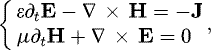 (1)
where ϵ is the permittivity of the medium, μ its permeability. In a conductive medium, J = σE, with σ the conductivity.
(1)
where ϵ is the permittivity of the medium, μ its permeability. In a conductive medium, J = σE, with σ the conductivity.
The discontinuous Galerkin method is introduced for solving the conservative form of partial differential equations. This method consists in discretizing the variational formulation of (1) on each mesh element T of the domain  :
:
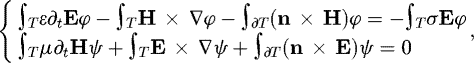 (2)
where φ and ψ are test functions. In each T, a finite element method is applied and a mapping technique is employed to facilitate the use of high order mesh elements. The interface terms (n × H) and (n × E) are replaced by numerical flux expressions
(2)
where φ and ψ are test functions. In each T, a finite element method is applied and a mapping technique is employed to facilitate the use of high order mesh elements. The interface terms (n × H) and (n × E) are replaced by numerical flux expressions  and
and  as in a finite volume method. Different formulations of the flux expressions exist [9]. These following expressions (3) resulting in different numerical schemes are implemented. For α = 0, centered fluxes are obtained and numerical schemes are dispersive. For α = 1, upwind fluxes are obtained and numerical schemes are dissipative. We have
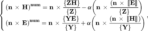 (3)where
  , Y = 1/Z,
 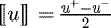 , and
, and 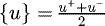 . The superscript “−” denotes the values for fields in the current element, while “+” is for the adjacent element. In this work, the upwind fluxes are considered, the time integration is ensured by an explicit four stages Runge-Kutta method (RK44) and the spatial discretization is performed with the third order tetrahedral mesh elements to improve accuracy of the results.
2.2 Numerical results
The coaxial cable model is designed by four concentric cylinders as shown in Figure 1a. At the center, the copper core diameter is 0.43 mm. The first layer of diameter 2.9 mm is the inner dielectric insulator whose relative permittivity is  . The second layer of diameter 3.2 mm is the woven copper shield whose conductivity is σ = 6.107 S/m−1. The third layer of diameter 3.6 mm is an outer plastic jacket whose relative permittivity is
  . The soft fault presented in Figure 1b is a partial chafing of the jacket, the shield, and the insulator on a length Lf, and the damaged depth of the dielectric insulator is noted as pf = 1 mm. Since a part of the field is radiated outside, a surrounding cylindrical vacuum volume is added with perfectly matched layers to operate like free space as in experimental measurements [10].
The simulation consists in injecting a Gaussian pulse of frequency band [0, 7]GHz in the cable. The incident radial electric field is given by: 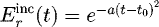 with a = 3.1020 and
  . The reflected field is recorded on an observation plane S located in front of the soft fault. It is computed as
 (4)
(4)
Two lengths Lf = {5, 7.5} cm are considered and the impulse responses versus the position z = 2vt, with  , are presented in Figure 2. For each case, the first reflection is positive and the second is negative. This is due to the higher wave velocity value in the defective zone. The distance between the positive and negative peaks is equal to the length of the damaged part. The amplitudes of the negative pulses are lower than those of the positive pulses. This is due to the radiated field outside the coaxial cable. When Lf increases the amplitude of the second reflection decreases because the field is radiated outside along the defective zone.
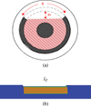 |
Fig. 1 Modeling of a damaged coaxial cable. (a) Section of the coaxial cable, (b) chafing of the shield and insulator. |
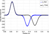 |
Fig. 2 Impulse responses of a chafing soft fault of length Lf = {5, 7.5} cm. |
3 Experimental approach
In this section we will focus on the comparison between the numerical simulation and the experimental results on chafing defects for diagnosis purposes. The early diagnosis of such defects is very important since they correspond to electrical wire damaged by abrasion against sharp edges caused by poor design, bad or broken holding of the cable. This results in a chafing of the insulator as modeled in the previous section and ultimately, in an extreme case where the insulator is completly removed over an angular portion, can lead to severe system failures.
3.1 Experimental setup
The experimental setup is shown in Figure 3. A faulty line is connected to a vector network analyzer through two  coaxial cables equipped with N connectors. The A and B fixtures are N to BNC coaxial adaptors. Since the SOLT (Short Open Load Thru) calibration is realized at the extremities of those cables, the position of the reference plane will be at the end of the cable connected to port 1. The scattering parameters are measured with an Agilent N9914 Fieldfox over a [0, 4]GHz range.
In this work, the faulty line including a chafing defect (Fig. 4) () is realized by partially milling the shielding and the insulator on a limited portion of a 60 cm,  RG58 coaxial cable, as shown in Figures 1 and 3. Two lengths Lf = {5, 7.5} cm with a depth d = 1 mm were realized.
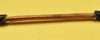 |
Fig. 3 A two port a vector network analyzer (VNA) is connected to a faulty line through the fixtures A and B. |
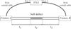 |
Fig. 4 The faulty line includes a chafing soft defect realized by partially removing by milling the shielding and the isolator. |
3.2 Experimental results
A common problem, when trying to characterize a soft defect on an electrical line by reflectometry, is that the fixtures at each extremity of the line also introduce insertion or return losses. In that case, the measured impulse responses also contains the signatures of the fixtures. Although very weak, the fixtures contribution cannot be neglected when dealing with soft defects since the perturbation they create on the line are of the same order of magnitude. In this work the two-window time gating method presented in Reference [6] is used to remove the contribution of the fixtures. It is based on the measurement of the four scattering parameters of the network and a selective gating of the mismatches caused by each fixture. Consequently the full de-embedding of the fixtures effect and the quantitative characterization of the signature of defects can be achieved. The result of the de-embedding process on the defective line is presented in Figure 5 and one can see that the contribution of the fixtures are mostly removed. Despite this technique, it remains a non-negligible noise level that leads on ripplings of the reflection coefficient in frequency domain.
To avoid these ripplings, a clean algorithm procedure [7] is applied in order to remove the noise and the unwanted inhomogeneities on the time domain impulse response. In this work, the shape of the impulse response at one interface of the defect can not be considered as a sinc function. As a matter of fact, the leakage of the field with frequency will affect the reflection coefficient and consequently the shape of the impulse response. The interface impulse response used in the clean algorithm procedure was taken as the main lobe of the first reflection (Fig. 6).
Figure 7 shows the comparison of the reflection coefficients between the experimental measurements and the numerical model for Lf = {5, 7.5} cm. The error over frequency is around 5% below 1.5 GHz and increases with frequency since many experimental parameters can have an influence on the losses. The reflection coefficient obtained from a chain matrix model, that consists in a transmission line model with the three sections cascaded, is also added for Lf = 7.5 cm. This chain matrix model does not take into account the losses due to the leakage in the outer medium, and can account for the model of a crushing defect where the shielding would not have been damaged. The periodicity of the lobes with frequency is in very good agreement but this result more importantly clearly emphasizes the effect of the losses on the frequency response. Consequently, the specific signature of the chafing defect evidenced here is very important since it allows us to discriminate a simple crushing defect (no leakage, no short circuit risk) from a chafing defect potentially more severe. The length of the defect can be estimated through the measurement of lobes periodicity and the identification of the nature of the defect through the recognition of the attenuation pattern by cross correlation analysis.
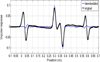 |
Fig. 5 Original and de-embedded impulse responses of a defective line under test. The line is a 60 cm 50Ω RG58 coaxial cable including a 7.5 cm chafing defect. |
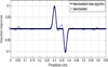 |
Fig. 6 Result of the de-embedding and clean algorithm procedure on the impulse responses of the defective line under test with a chafing defect of length Lf = 7.5 cm. |
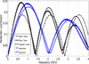 |
Fig. 7 Comparison of reflection coefficient between the experimental measurements, the numerical DG model and a simple chain matrix model for Lf = 7.5 cm and d = 1 mm. |
4 Conclusion
A numerical model, as well as an experimental validation, of chafing soft defects on an electrical line was presented. The model is based on the implementation of the discontinous Galerkin method and the defects created by milling coaxial cables were characterized by time and frequency domain reflectometry. A de-embeding and clean algorithm procedure was also used in order to denoise, extract, and quantitatively identify the signature of the soft defect. The method is very efficient and, for the first time to our knowledge, a frequency signature allowing to discriminated a crushing from a chafing defect was evidenced. This result can be a powerful tool for the preventive diagnosis and maintenance of potentially severe soft defects.
References
- F. Auzanneau, Prog. Electromagn. Res. B 49, 253 (2013) [CrossRef] [Google Scholar]
- M. Franchet, N. Ravot, O. Picon, IEEE Electromagn. Compat. Mag. 2, 54 (2013) [Google Scholar]
- F. Loete, Q. Zhang, M. Sorine, IEEE Trans. Antennas Propag. 63, 2532 (2015) [Google Scholar]
- E.J. Lundquist, J.R. Nagel, S. Wu, B. Jones, C. Furse, IEEE Sens. J. 13, 1172 (2013) [Google Scholar]
- A. Manet, A. Kameni, F. Loete, G. Genoulaz, L. Pichon, O. Picon, IEEE Trans. Electromagn. Compat. 59, 533 (2017) [Google Scholar]
- G. Gronau, I. Wolff, IEEE Trans. Microw. Theory Tech. 37, 479 (1989) [Google Scholar]
- C. Buccella, M. Feliziani, G. Manzi, IEEE Trans. Electromagn. Compat. 46, 597 (2007) [Google Scholar]
- A. Kameni, A. Modave, M. Boubekeur, V. Preault, L. Pichon, C. Geuzaine, Eur. Phys. J. Appl. Phys. 64, 24508 (2013) [CrossRef] [EDP Sciences] [Google Scholar]
- J.S. Hesthaven, T. Warburton, J. Comput. Phys. 181, 186 (2002) [Google Scholar]
- A. Modave, A. Kameni, J. Lambretchs, E. Delhez, L. Pichon, C. Geuzaine, Eur. Phys. J. Appl. Phys. 64, 24502 (2013) [CrossRef] [EDP Sciences] [Google Scholar]
Cite this article as: Abelin Kameni, Florent Loete, Lionel Pichon, Time domain reflectometry model: analysis and characterization of a chafing defect in a coaxial cable, Eur. Phys. J. Appl. Phys. 83, 30601 (2018)
All Figures
|
Fig. 1 Modeling of a damaged coaxial cable. (a) Section of the coaxial cable, (b) chafing of the shield and insulator. |
| In the text | |
|
Fig. 2 Impulse responses of a chafing soft fault of length Lf = {5, 7.5} cm. |
| In the text | |
|
Fig. 3 A two port a vector network analyzer (VNA) is connected to a faulty line through the fixtures A and B. |
| In the text | |
|
Fig. 4 The faulty line includes a chafing soft defect realized by partially removing by milling the shielding and the isolator. |
| In the text | |
|
Fig. 5 Original and de-embedded impulse responses of a defective line under test. The line is a 60 cm 50Ω RG58 coaxial cable including a 7.5 cm chafing defect. |
| In the text | |
|
Fig. 6 Result of the de-embedding and clean algorithm procedure on the impulse responses of the defective line under test with a chafing defect of length Lf = 7.5 cm. |
| In the text | |
|
Fig. 7 Comparison of reflection coefficient between the experimental measurements, the numerical DG model and a simple chain matrix model for Lf = 7.5 cm and d = 1 mm. |
| In the text | |
Current usage metrics show cumulative count of Article Views (full-text article views including HTML views, PDF and ePub downloads, according to the available data) and Abstracts Views on Vision4Press platform.
Data correspond to usage on the plateform after 2015. The current usage metrics is available 48-96 hours after online publication and is updated daily on week days.
Initial download of the metrics may take a while.